This article is about a review of the paper [1], and is the first part of a personal research project to apply Graph Neural Network (GNN) to the field of cascading outage prediction or detection.

The primary purpose is to create large-scale datasets for training GNN-based models through the cascading outage simulator presented in this paper.

Research Project’s Git Repository

1. CASCADING OUTAGE SIMULATOR

WHAT & WHY

The importance of studying cascading outages has been recognized [2]-[4]. However, since electrical power networks are very large and complex systems [5], understanding the many mechanisms by which cascading outages propagate is challenging [1].

Cascading outage simulators are designed to set and reproduce scenarios that can occur in the electric grid, and it allow us to study a wide variety of different mechanisms of cascading outages.

IN THE PAPER

The paper presents the design of and results from a new non-linear dynamic model of cascading failure in power system, called “Cascading Outage Simulator with Multi-process Integration Capabilities” (COSMIC).

In COSMIC [1], …

Dynamic components are modeled using differential equations.
Power flows are represented using non-linear power flow equations.
Discrete changes (e.g., components failures, load shedding) are described by a set of equations (constraints).

COSMIC has the following benefits [1].

It provids an open platform for research and development.
The dynamic/adaptive time step and recursive islanded time horizons implemented in this simulator which allows for faster computations during, near, steady-state regimes, and fine resolution during transient phases.
It can be easily integrated with High Performance Computing (HPC) clusters to run many simulations simultaneously at a much lower cost.

2. HYBRID SYSTEM MODELING IN COSMIC

A. Hybrid differential-algebraic formulation

Dynamic power networks are modeled as sets of DAEs. Each DAE is composed of three parts:

  i. A set of Differential equations
  ii. A set of Algebraic equations
  iii. A set of Constraints

i. A set of Differential equations

\[\frac{d\mathbf{x}}{dt}=\mathbf{f}(t, \mathbf{x}(t), \mathbf{y}(t), \mathbf{z}(t)) \tag{1}\]

$\mathbf{x}$ is a vector of continuous state variables that change with time according to a set of differential equations.
(1) represent the machine dynamics (APPENDIX - A).

ii. A set of Algebraic equations

\[\mathbf{g}(t, \mathbf{x}(t), \mathbf{y}(t), \mathbf{z}(t)) =0 \tag{2}\]

$\mathbf{y}$ is a vector of continuous state variables that have pure algebraic relationships to other variables in the system.
(2) encapsulate the standard ac power flow equations (APPENDIX - B).
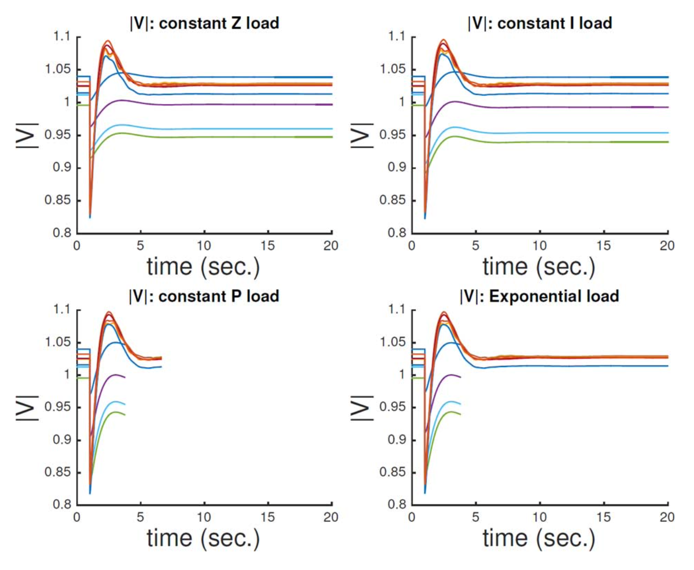
(2) is largely dependent on the load models (Figure 1. ZIPE models).

Q. WHAT IS EXPONENTIAL MODEL???

Figure 1. Illustrates a dramatic impact of load models on algebraic convergence. [1]

iii. A set of Constarints

\[\mathbf{h}(t, \mathbf{x}(t), \mathbf{y}(t), \mathbf{z}(t))<0 \tag{3}\]

$\mathbf{z}$ is a vector of state variables (relay status) that can only take integer states $( z_i ∈ [0, 1])$.
(3) represent the constraints.
If a constraint $\mathbf{h_i}(…)<0$ fails (outage occurs), an associated counter function $\mathbf{d_i}$ (relay) activates.

cf. What happens during cascading failures?

During cascading failures, power systems many undergo discrete changes. The discrete event(s) will consequently change the systems dynamic response and algebraic equations, which may result in cascading failures, system islanding, and large blackouts.

B. Relay modeling

Major disturbances cause system oscillations, and these oscillations may naturally die out as the system adjusts to a new equilibrium. In order to ensure that relays do not trip due to brief transient state changes, time-delays are added to each protective relay in COSMIC.

Five types of protective relays are modeled in COSMIC:

Over-current (OC) relays
Distance (DIST) relays
Temperature (TEMP) relays
Under-voltage load shedding (UVLS) relays
Under-frequency load shedding (UFLS)

C. Solving the hybrid DAE

COSMIC used the following two strategies to solve the hybrid DAE.

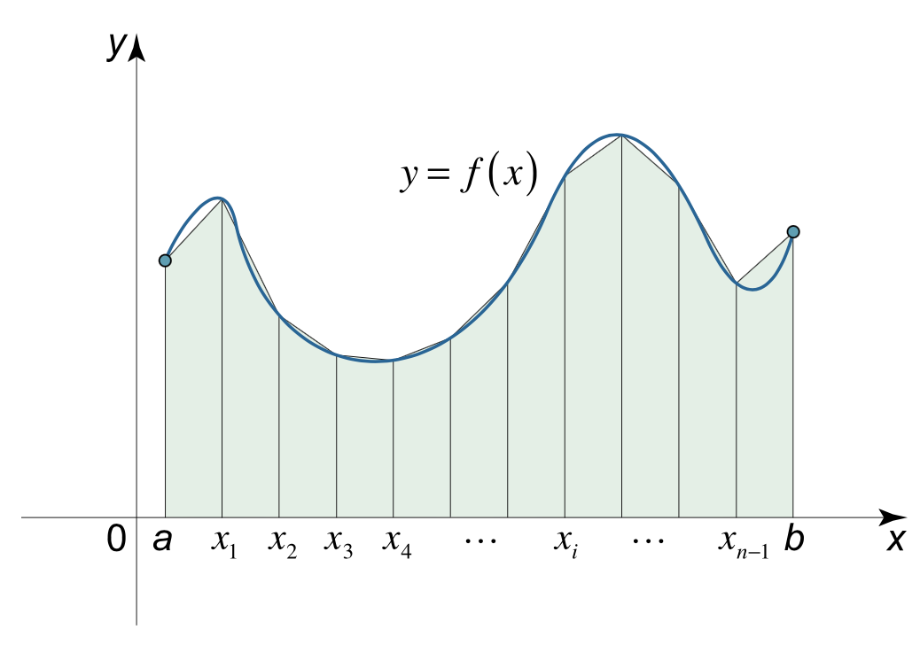
COSMIC uses the trapezoidal rule to simultaneously integrate and solve the differential and algebraic equations.
COSMIC implements a variable time-step size in order to trade-off between the diverse time-scales of the dynamics.
- During transition periods: small step size → fine resolution.
- During steady-state periods: large step size → faster computation.

Trapezoidal Rule

\[\int_{a}^{b} f(x) \,dx = \frac{\Delta x}{2}[f(x_0) + 2f(x_1) +... + 2f(x_{n-1}) + f(x_n)]\]

DAE during discrete event

\[0 = \mathbf{x} + \frac{t_d-t}{2} [\mathbf{f}(t)+\mathbf{f}(t_d, \mathbf{x}_d, \mathbf{y}_d, \mathbf{z}_d)] \tag{4}\]

Q. HOW TO APPLY TRAPEZOIDAL RULE TO A DISCRETE POINT???

\[0=\mathbf{g}(t_d, \mathbf{x}_+, \mathbf{y}_+, \mathbf{z}) \tag{5}\] \[0>\mathbf{h}(t_d, \mathbf{x}_+, \mathbf{y}_+) \tag{6}\] \[0=\mathbf{d}(t_d, \mathbf{x}_+, \mathbf{y}_+) \tag{7}\]

where

$t$ is the previous time point.
$t_d$ is the point a discrete event occurs.

Because of the adaptive time step size, COSMIC retains $t_d$ from $t_d = t + \Delta t_d$, in which $\Delta t_d$ is found by linear interpolation of two time steps.

Q. HOW THE LINEAR INTERPOLATION WORKS IN HERE???

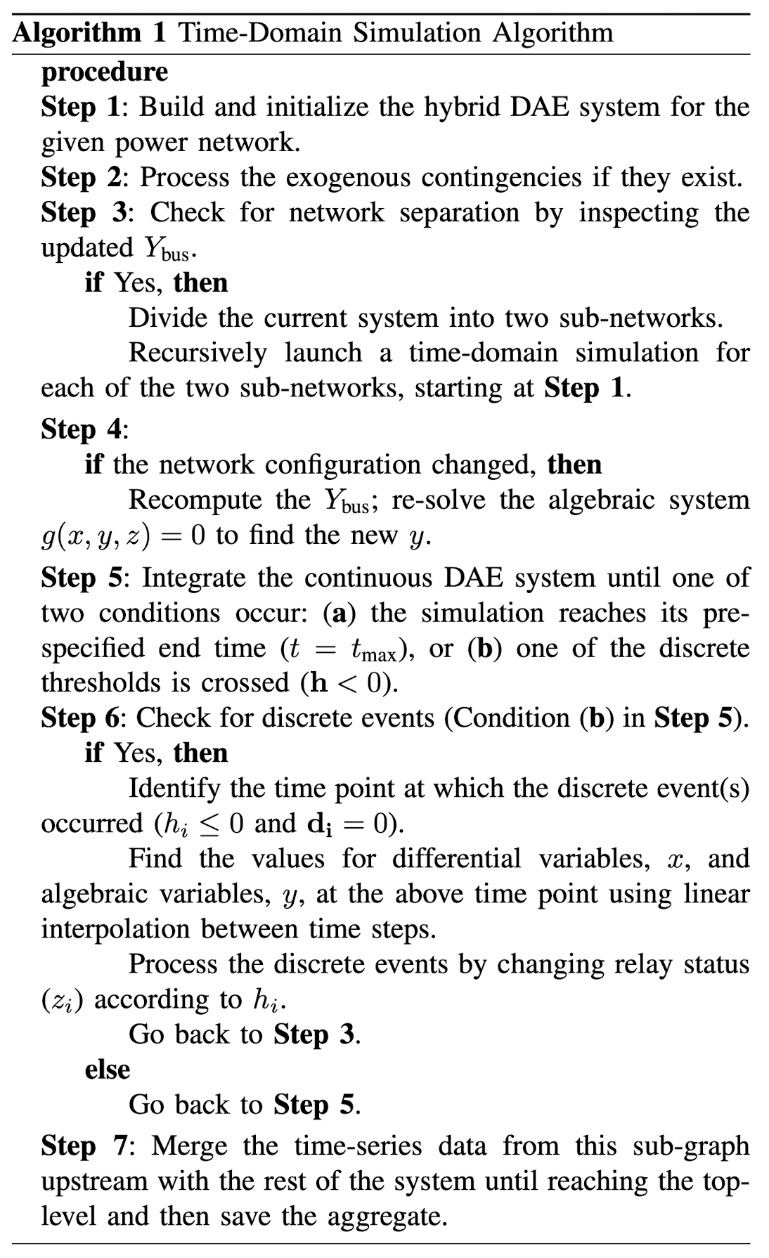
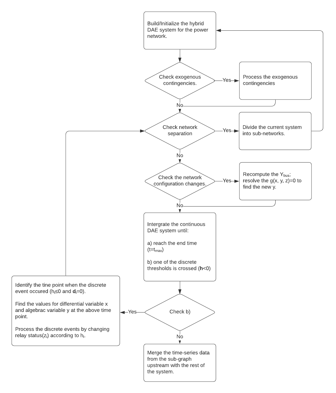
Time-Domain Simulation Algorithm

The description of Time-Domain Simulation Algorithm implemented in COSMIC and a corresponding flowchart are as follows.

The feature of this algorithm that we need to focus is that when network separation occurs, each subnetwork is computed independently in a recursive manner.

Figure 3. Time-Domain Simulation Algorithm [1]

Figure 4. Flowchart of Time-Domain Simulation Algorithm

3. EXPERIMENTS AND RESULTS

In this paper, the performance and characteristics of COSMIC were explored through several experiments as follows.

A. Polar formulation vs. Rectangular formulation in computational efficiency

Purpose

To compare the computational efficiency of the polar and rectangular formulations of the model.

Q. WHY DO WE NEED TO COMPARE THE PERFOMANCE BETWEEN RECT AND POLAR???

Used test systems

39-bus system
2383-bus system

Results

On Table I, in 39-bus case, the rectangular formulation required fewer linear solves for different demand losses.
On Table II, in 2383-bus case, there was no significant improvement for the rectangular formulation over the polar formulation, and the number of linear solves that resulted from both forms were almost identical.

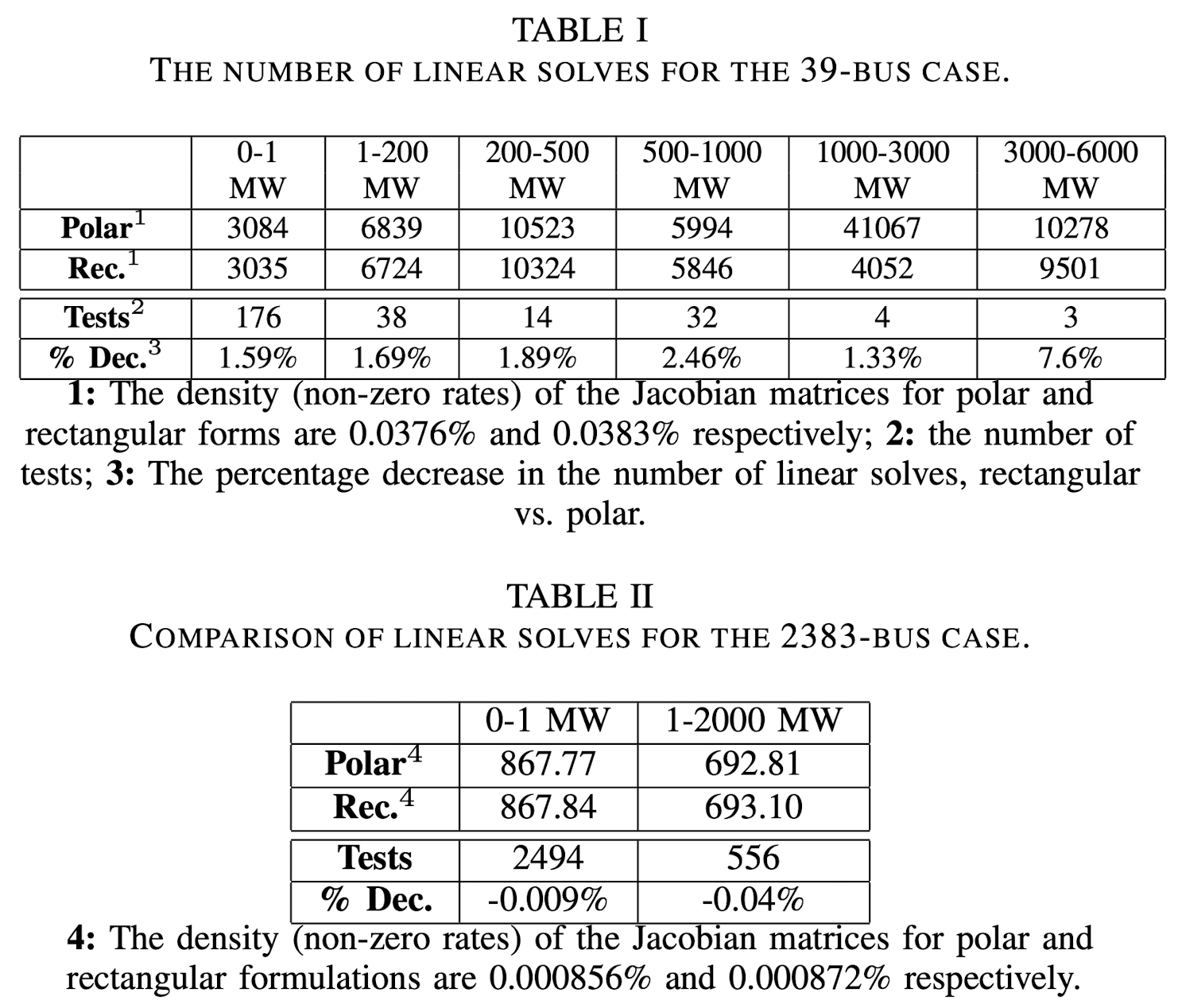
Table I & Table II. Performance comparison between Rect & Polar [1]

Q. WHY DO WE NEED TO KNOW ABOUT THE DENSITY OF THE JACOBIAN MATRICES???

B. Relay event illustration

Purpose

To illustrate the different relay functions implemented in COSMIC and their time delay algorithms.

Used test systems

9-bus system

Results

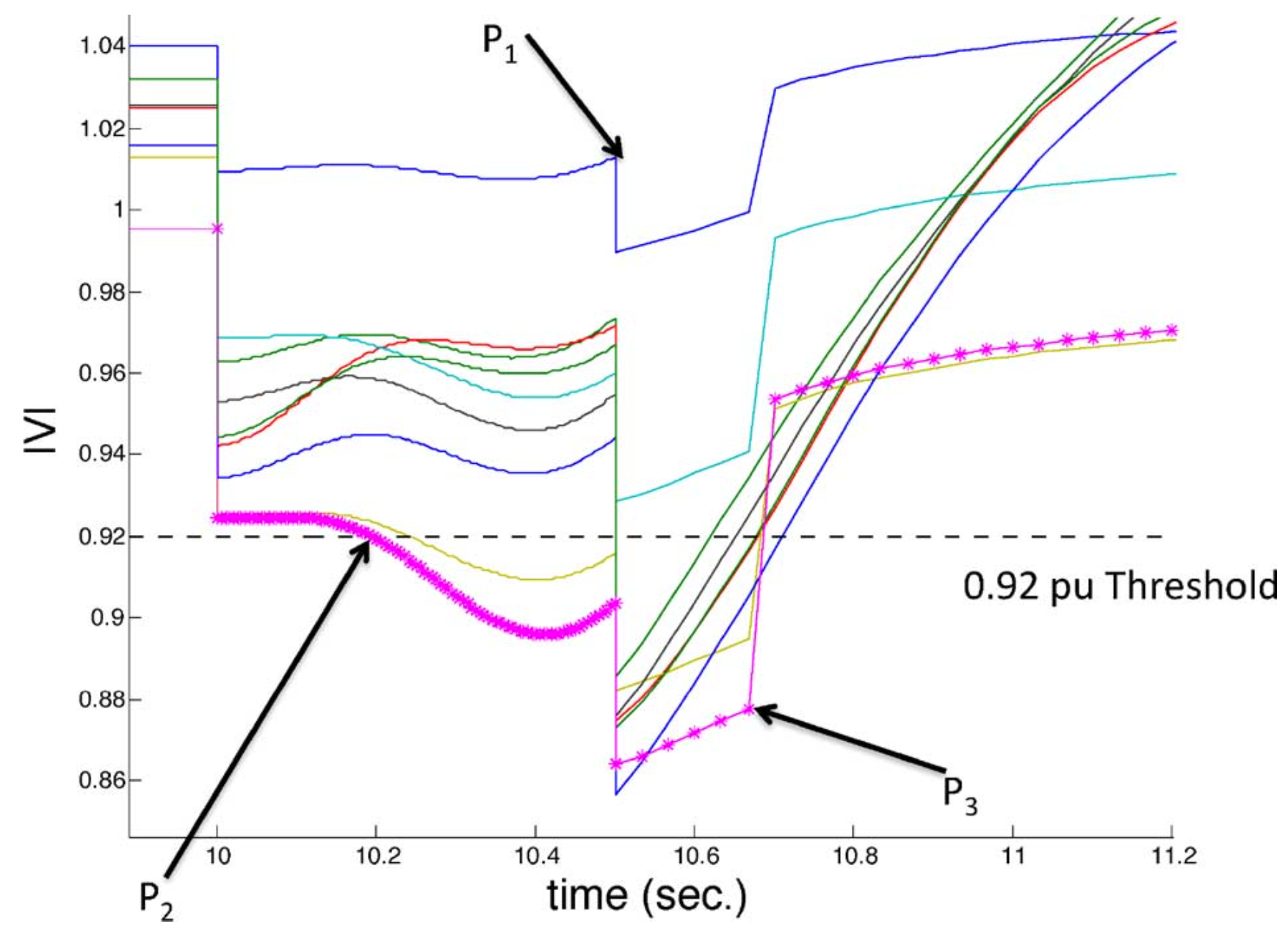
Figure 5. Bus voltage magnitudes when the branch from bus 6 to bus 9 in the 9-bus system is tripped. [1]

A single-line outage was occurred at $t=10$ seconds, and DIST relay timer activate.
$t_{preset-delay}=0.5$
$P_1 (t=10.5)$: $t_{delay}$ ran out, and another line outage was occurred.
$P_2$: the magenta voltage trace violated the limit, and UVLS relay timer activate.
$P_3$: UVLS relay took action and shed 25% of the initial load at the bus.

C. Cascading outage examples

Purpose

To demonstrates how COSMIC processes cascading events such as line branch outages, load shedding, and is-landing.

Used test systems

39-bus system
2383-bus system

Results

39-Bus Case

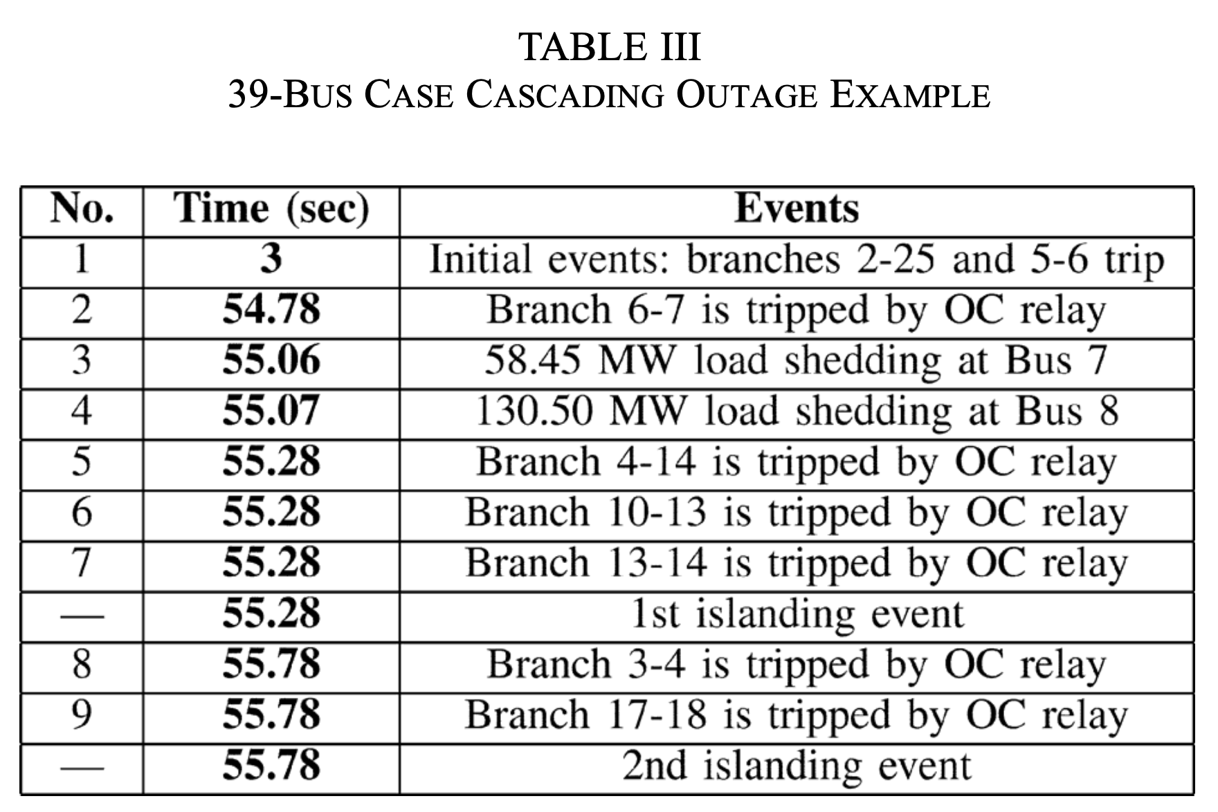
At $t=3.00$ sec, the system suffered a strong dynamic oscillation after the initial two exogenous events (branches 2–25 and 5–6).
At $t=54.06$ sec, the first OC relay at branch 4–5 triggered.
At $t=55.06$ and $t=55.07$ sec, load shedding at two buses (Bus 7 and Bus 8) occurred.
At $t=55.28$ sec, another two branches (10–13 and 13–14) shut down after OC relay trips. These events separated the system into two islands.
At $t=55.78$ sec, two branches (3–4 and 17–18) were taken off the grid and this resulted in another island. The system eventually ended up with three isolated networks.

2383-Bus Case

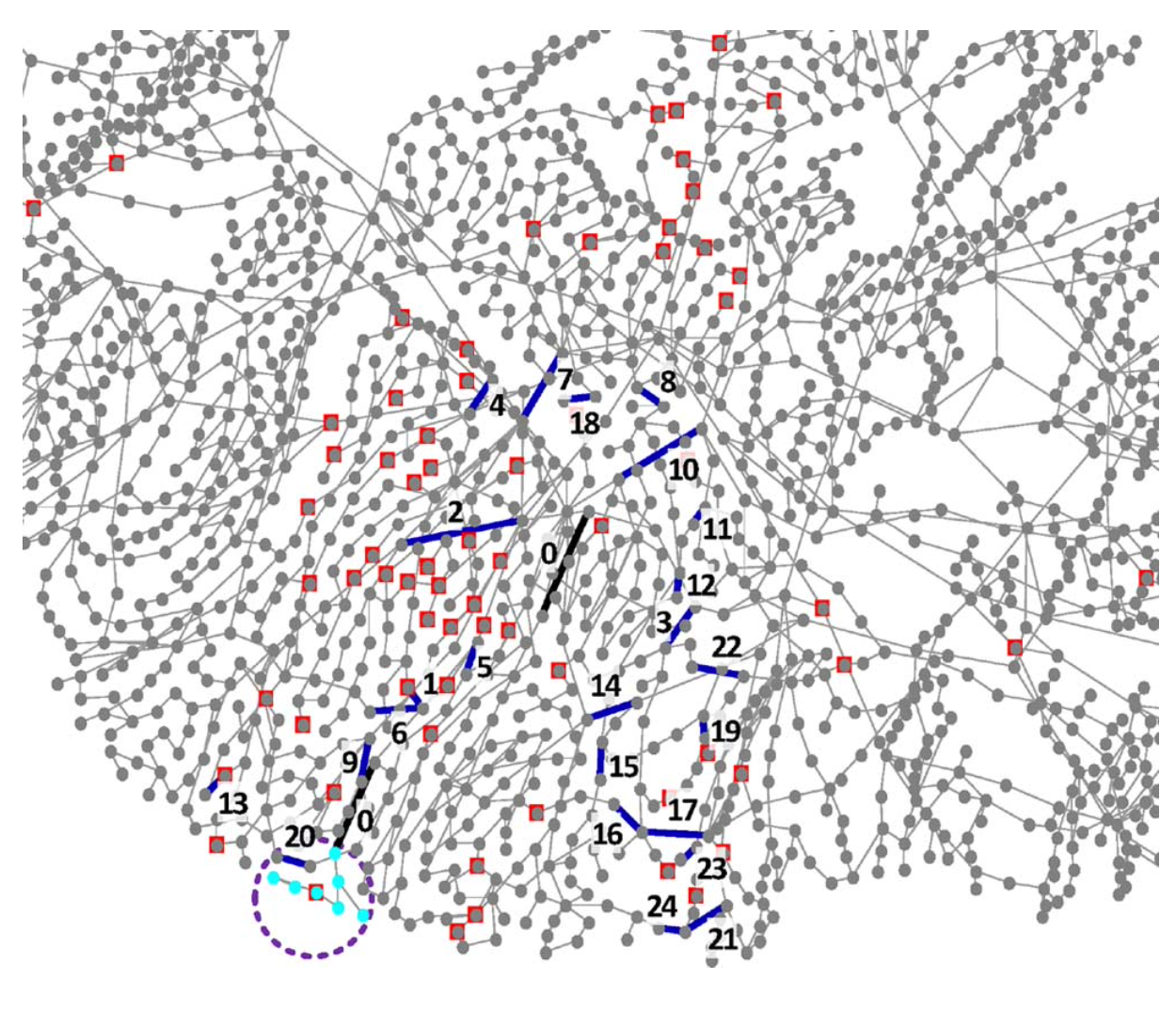
Number 0 with black highlights denotes the two initial events (N-2 contingency).
Other sequential numbers indicate the rest of the branch outages.
In this example, 24 branches are off-line and cause a small island (within the dashed circle) in the end.
The dots with additional red squares indicate buses where load shedding happens.

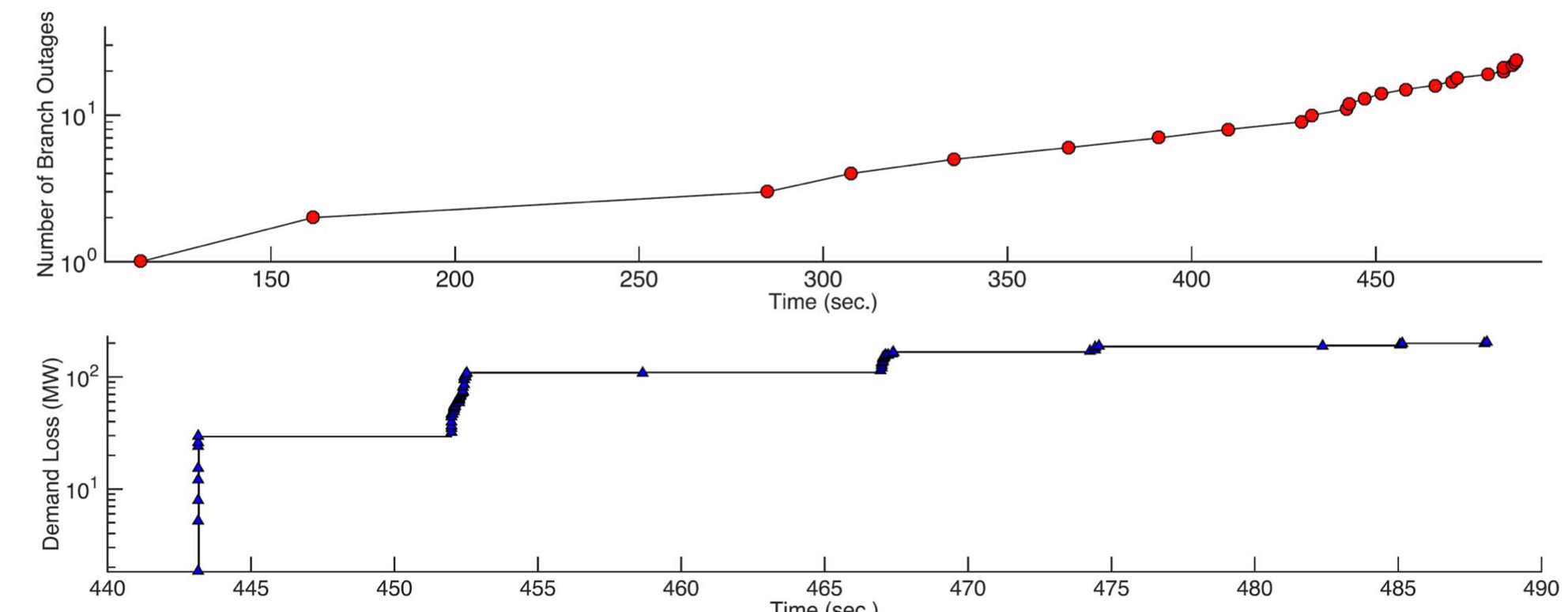
Figure 7. Branch outage events & Load-shedding events listed in Figure 8 [1]

The top panel in Figure 7 shows the timeline of all branch outage events for the 2383-bus cascading scenario, and the lower panel zooms in the load-shedding events.

What we found here are …

In the early phase of this cascading outages, the occurrence of the components failed relatively slowly, but it speeds up as the number of failures increased (check top panel).
When the system condition was substantially compromised, fast collapse occurs and the majority of the branch undergo outages as well as the load shedding events (check lower panel).

D. N-2 contingency analysis

Purpose

To studies the impact of different load modeling assumptions on cascading failure sizes.

Used test systems

2383-bus system

Results

Demand Loss

Figure 10 shows the complementary cumulative distribution function (CCDF) of demand losses for these four groups of simulations.

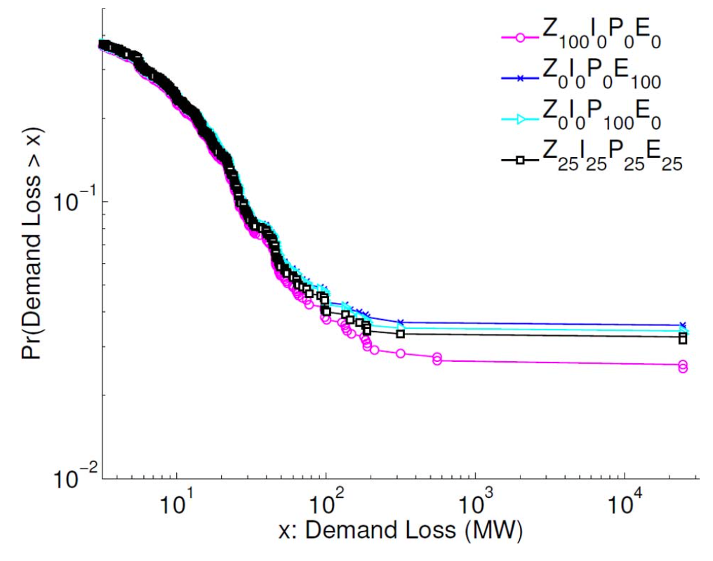
The CCDF plots of demand losses exhibit a heavy-tailed blackout size distribution, which are typically found in both historical blackout data and cascading failure models [7].

Q. WHY A HEAVY-TAILED DIST IS EASILY FOUND IN HISTORICAL DATA AND CASCADING FAILURE MODELS???

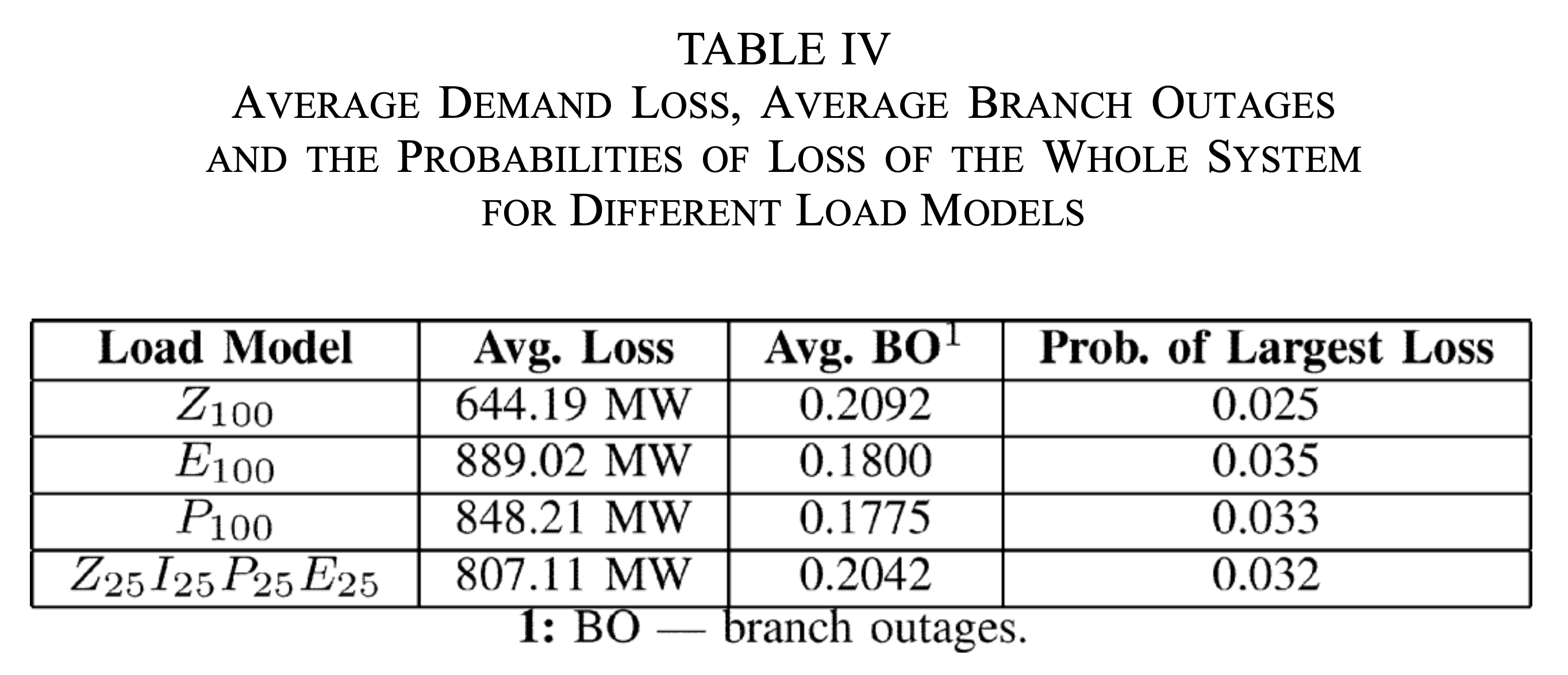
Table IV. Average demand loss, average branch outages, and the probabilityies of loss for different load models [1]

The constant Z load model ($Z_{100}I_0P_0E_0$) shows the best performance based on the average power loss and the probability of large blackout (listed in Table IV).
As can be seen in Table IV, the probabilities of large demand losses varies from 2.5% to 3.5% for those four load configurations.
These results show that load models play an important role in dynamic simulation and may increase the frequency of nonconvergence if they are not properly modeled.

Q. WHAT IS THE EXACT MEANDING OF NOT PROPERLY MODELED???

E. Comparison with a dc cascading outage simulator

Purpose

To compare results from COSMIC with results from a dc-power flow based model of cascading failure.
It will help us to understand similarities and differences between these two different modeling approaches.

Used test systems

2383-bus system

Results

The probabilities of demand losses

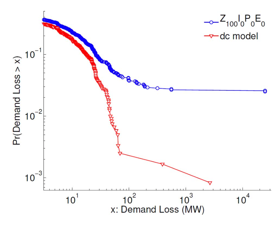
Figure 9. CCDF Demand Loss for COSMIC & DC Simulator [1]

The probability of demand losses in the dc simulator is lower than that of COSMIC for the same amount of demand losses.
The dc model is much more stable and does not run into problems of numerical nonconvergence.
COSMIC assumes that the network or sub-network in which the numerical failure occurred experienced a complete blackout.
As a result, numerical failures in solving the DAE system greatly contributed to the larger blackout sizes. → It may deteriorate the accuracy.

DC model

Pros
- It is numerically stable, making it possible to produce results that can be statistically similar to data from real power systems [8].
Cons
- It includes numerous simplifications that are substantially different from the “real” system.

Dynamic model

Pros
- It includes many mechanisms of cascading that cannot be represented in the dc model.
Cons
- It needs many assumptions that are needed substantially impact the outcomes, potentially in ways that are not fully accurate.

Path Agreement Measurement [9]

\[R(m_1, m_2) = \sum_{i=1}^{|C|}\frac{1}{C} \frac{|A_i \cap B_i|}{|A_i \cup B_i|} \tag{8}\]

where

models $m_1$ and $m_2$ are both subjected to the same set of exogenous contingencies $C=${$c_1,c_2,…$}.
It measures the average agreement in the set of dependent events that result from each contingency in each model.

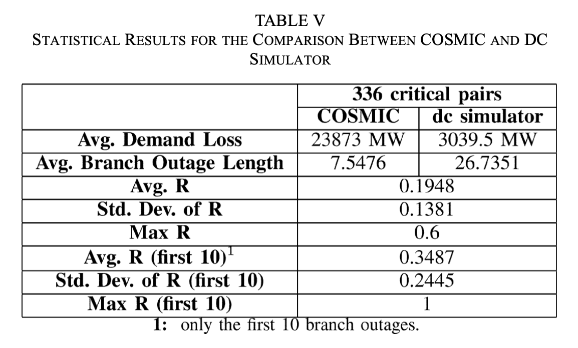
Table V. Statical Results for the Comparison between COSMIC & DC Simulator [1]

Table V shows that the average between the two models for the whole set of sequences is 0.1948, which means that there are substantial differences between cascade paths in the two models.
Part of the reason is that the dc model tends to produce longer cascades and consequently increase the denominator in (8).

Q. WHY DC MODEL TENDS TO PRODEUCE LONGER SCENARIOS???

In order to control this, we computed only for the first ten branch outage events (early stage).
The average R increased to 0.3487, and some of the cascading paths showed a perfect match ($R=1$).
This suggests that the cascading paths resulting from the two models tend to agree during the early stages of cascading, when nonlinear dynamics are less pronounced, but disagree during later stages.

4. CONCLUSION

Through the above experiments, the following conclusions are drawn.

COSMIC represents a power system as a set of hybrid discrete/continuous differential algebraic equations, simultaneously simulating protection systems and machine dynamics.
From the N−2 contingency analysis, we found that COSMIC produces heavy-tailed blackout size distributions, which are typically found in both historical blackout data and cascading failure models [7] (Figure 8).
From the N−2 contingency analysis, we found that the blackout size results show that load models can substantially impact cascade sizes (Table IV).
From the comparison with a dc cascading outage simulator, we found that the relative frequency of very large events may be exaggerated in dynamic model due to numerical non-convergence (about 3% of cases).
From the comparison with a dc cascading outage simulator, we found that the two models largely agreed for the initial periods of cascading (for about 10 events), then diverged for later stages where dynamic phenomena drive the sequence of events.
Detailed dynamic models of cascading failure can be useful in understanding the relative importance of various features of these models.

5. MY RESEASRCH PROJECT

Purpose / Goal

Forecast or detect (in real-time) cascading outages in power systems.

Approach

Use a GNN based model to predict or detect cascading outages.

Experiments

Step 1. Data Generation

Need to introduce randomness to create large size of dataset.
Randomness will be given by the method that generated the uncertain loads in [10]:

\[d := d + \mathcal{N}(\mu=0, \sigma = 0.03 * d)\]
- $d$ is a load.
- $\mathcal{N}$ is normal distribution with mean zero and standard deviation proportional to the load.

Q. WHICH FEATURES (e.g. $P_d, Q_d, P_g, Q_g$ or outage event time $t_{event}$) SHOULD BE GIVEN RANDOMNESS?

Codes

Step 2. Design the GNN Model Architecture

Does the model ARCHITECTURE is proper for the GOAL?
What is the STRENGTH of the model ARCHITECTURE? and WHY?

Step 3. Train & Test the Model

Step 4. Tune the Hyper-parameters

🤔

Results (What we want to see…)

High enough prediction or detection accuracy.
Extremely high computational efficiency compared to old methods.
A GNN based model having significantly fewer nodes (trainable parameters) than other deep learning models.

6. APPENDIX

A. Differential equations in dynamic power system [1]

Equation for rotor speed

\[M \frac{dw_i}{dt} = P_{m,i} - P_{g,i} - D(w_i-1)\]

where

$\forall i \in N_G$ ($N_G$ is the set of all generator buses).
$M$ is a machine inertia constant.
$w_i$ is a rotor speed.
$P_{m,i}$ is the mechanical power input.
$P_{g,i}$ is the generator power output.
$D$ is a daping constant.

Equation for rotor angle

\[\frac{d\delta_i(t)}{dt} = 2 \pi f_0 (w_i-1)\]

where

$delta_i(t)$ is the rotor angle.
$f_0$ is the nominal frequency.
$w_i$ is fortor speed.

etc.

B. AC power flow equation [11]

Relation between following three compenets.

real/reactive power injected into each bus ($P_i, Q_i; i=1, 2, …, n$)
bus voltage magnitude of each bus ($V_i; i=1, 2, …, n$)
phase angle of each bus ($\theta_i; i=1, 2, …, n$).

\[P_i = V_i\sum_{k=1}^{n}\{ G_{ik} cos(\theta_i-\theta_k) +B_{ik}sin(\theta_i-\theta_k) \}\] \[Q_i = V_i\sum_{k=1}^{n}\{ G_{ik} sin(\theta_i-\theta_k) +B_{ik}cos(\theta_i-\theta_k) \}\]

where

$n$ is the number of buses of the system.
$Y_{ik} = G_{ik} + j B_{ik}$ is (i, k)-th entry of Y-bus matrix.

REFERENCES

[1] J. Song, E. Cotilla-Sanchez, G. Ghanavati and P. D. H. Hines, “Dynamic Modeling of Cascading Failure in Power Systems,” in IEEE Transactions on Power Systems, vol. 31, no. 3, pp. 2085-2095, May 2016.

[2] M. Papic et al., “Survey of tools for risk assessment of cascading outages,” in Proc. IEEE Power and Energy Soc. General Meeting, 2011, pp. 1–9.

[3] M. Vaiman et al., “Risk assessment of cascading outages: methodologies and challenges,” IEEE Trans. Power Syst., vol. 27, no. 2, pp. 631–641, May 2012.

[4] I. Dobson, B. A. Carreras, V. E. Lynch, and D. E. Newman, “Complex systems analysis of series of blackouts: cascading failure, critical points, and self-organization,” Chaos: Interdisciplinary J. Nonlinear Sci., vol. 17, no. 2, p. 026103, 2007.

[5] M. Eppstein and P. Hines, “A ‘random chemistry’ algorithm for identifying collections of multiple contingencies that initiate cascading failure,” IEEE Trans. Power Syst., vol. 27, no. 3, pp. 1698–1705, Aug. 2012.

[6] “Trapezoidal Rule,” Math24, 30-Apr-2020. [Online]. Available: https://www.math24.net/trapezoidal-rule/. [Accessed: 07-Jan-2021].

[7] P. Hines, J. Apt, and S. Talukdar, “Large blackouts in North America: historical trends and policy implications,” Energy Policy, vol. 37, no. 12, pp. 5249–5259, 2009.

[8] B. A. Carreras, D. E. Newman, I. Dobson, and N. S. Degala, “Validating OPA with WECC data,” in 2013 46th Hawaii Int. Conf. on System Sciences (HICSS), Jan. 2013, pp. 2197–2204.

[9] R. Fitzmaurice, E. Cotilla-Sanchez, and P. Hines, “Evaluating the impact of modeling assumptions for cascading failure simulation,” in Proc. IEEE Power Energy Soc. General Meeting, Jul. 2012, pp. 1–8.

[10] D. Deka and S. Misra, “Learning for DC-OPF: Classifying active sets using neural nets,” 2019 IEEE Milan PowerTech, Milan, Italy, 2019, pp. 1-6.

[11] H.Zhu, “Lecture Note - Ch 06”, The University of Texas at Austin, Austin, TX, EE 369: POWER SYSTEMS ENGINEERING Course, Fall 2019