This article was written by referring to the Fall 2020 Numerical Analysis: Linear Algebra Course and the following links.
Gram–Schmidt Process
Given a set of linearly independent vectors $Span({ a_0, … , a_{n-1} } ) \subset \mathbb{C}^m$, the Gram-Schimdt process computes a new basis {$q_0, … , q_{n-1}$} that spans the same subspace as the original vectors, i.e. $Span({ a_0, … , a_{n-1} } ) = Span({ q_0, … , q_{n-1} } )$ [1].
It should be noted that we would like to have the new basis, ${ q_0, … , q_{n-1} }$, having the following characteristics.
- All vectors are unit vectors of length 1, i.e. $|q_i| = 1$.
- All vectors are mutually perpendicular, i.e. $q_i \perp q_j$ where $i \neq j$.
These characteristics can be obtained through the following routine which is composed by three steps [1]:
<Gram-Schmidt Process>
  Step 1. Compute the direction of the vectors.
  Step 2. Compute the magnitude of the normalizer.
  Step 3. Compute a unit vector.
- Compute the vector $q_0$ ($i=0$)
- Step 1. Compute the direction of the vectors.
- Stpe 2. Compute the magnitude of the normalizer.
- Step 3. Compute a unit vector.
- Result
- Compute the vector $q_1$ ($i=1$)
- Step 1. Compute the direction of the vectors.
- Step 2. Compute the magnitude of the normalizer.
- Step 3. Compute a unit vector.
- Result
- Compute the vector $q_2$ ($i=2$)
- Step 1. Compute the direction of the vectors.
- Step 2. Compute the magnitude of the normalizer.
- Step 3. Compute a unit vector.
- Result
- keep do the routine till $i=n-1$
- Step 1. Compute the direction of the vectors.
- Step 2. Compute the magnitude of the normalizer.
- Step 3. Compute a unit vector.
- Final Result
What we should pay attention to in the final result ($A = QR$) are …
- All column vectors of $Q$, the new basis {$q_0, … , q_{n-1}$}, are unit vector and mutually orthogonal, which means $Q$ is an unitary matrix.
- The matrix $R$ is upper triangular matrix and $rank(R)=m$.
- The dot product of $Q$ and $R$, which is equal to $A$, can be regarded as a linear combination of $Q$’s column vectors.
- The result of Gram-Shmidt Process can be regarded as a result of QR factorization (decomposotion).
Classical Gram-Schmidt (CGS)
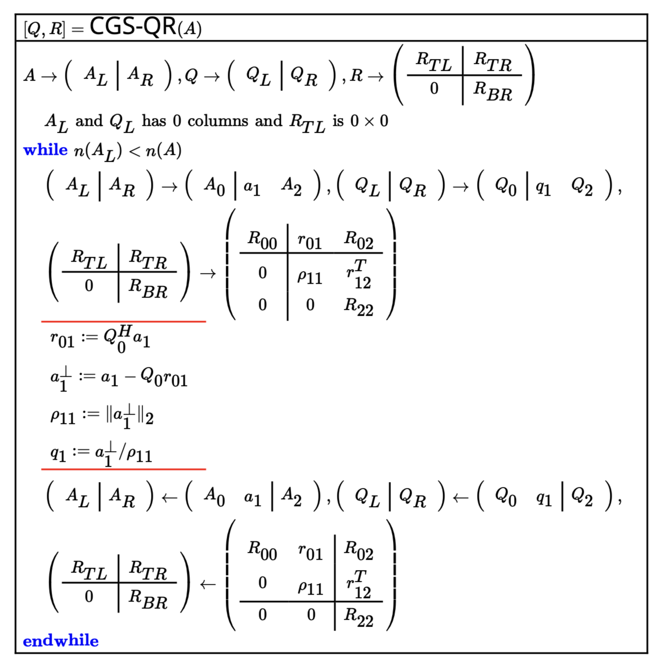
The content discussed in the previous section can be summarized into an algorithm as follows, which is the CGS-QR algorithm [2].
Consider $A=QR$.
Partition the given matrices as follows.
\[\left[\begin{array}{c|cc}A_{0} & a_{1} & A_{2}\end{array} \right]= \left[\begin{array}{c|cc}Q_{0} & q_{1} & Q_{2}\end{array} \right] \left[\begin{array}{c|cc} R_{0, 0} & r_{0, 1} & R_{0, 2} \\ \hline 0 & \rho_{1, 1} & r_{1, 2}^T\\ 0 & 0 & R_{2, 2} \end{array} \right]\]Assume that $Q_0$ and $R_{0,0}$ have already been computed.
Since $Q$ is unitary matric ($Q_0^HQ_0=I$ and $Q_0^Hq_1=0$),
- $Q_0^Ha_1=Q_0^HQ_0r_{0,1}+q_1\rho_{1,1}=r_{01}$
Compute $r_{0,1}$, which is already known.
- $r_{0,1}:=Q_0^Ha_1$
Compute $a_1^\perp$ and $\rho_{1,1}$ (Step 1. & 2.).
- $a_1^\perp:=a_1-Q_0r_{0,1}$
- $\rho_{1,1}:=|a_1^\perp|$
Compute $q_1$ (Step 3.).
- $q_1 := a_1^\perp / \rho_{1,1}$
Figure 1. shows Classical Gram-Schmidt algorithm for computing the QR factorization of a matrix A. The algorithm used FLAME notation.
Code 1. shows the algorithms in python language.
Code. 1: CGS QR in python
Modified Gram-Schmidt (MGS)
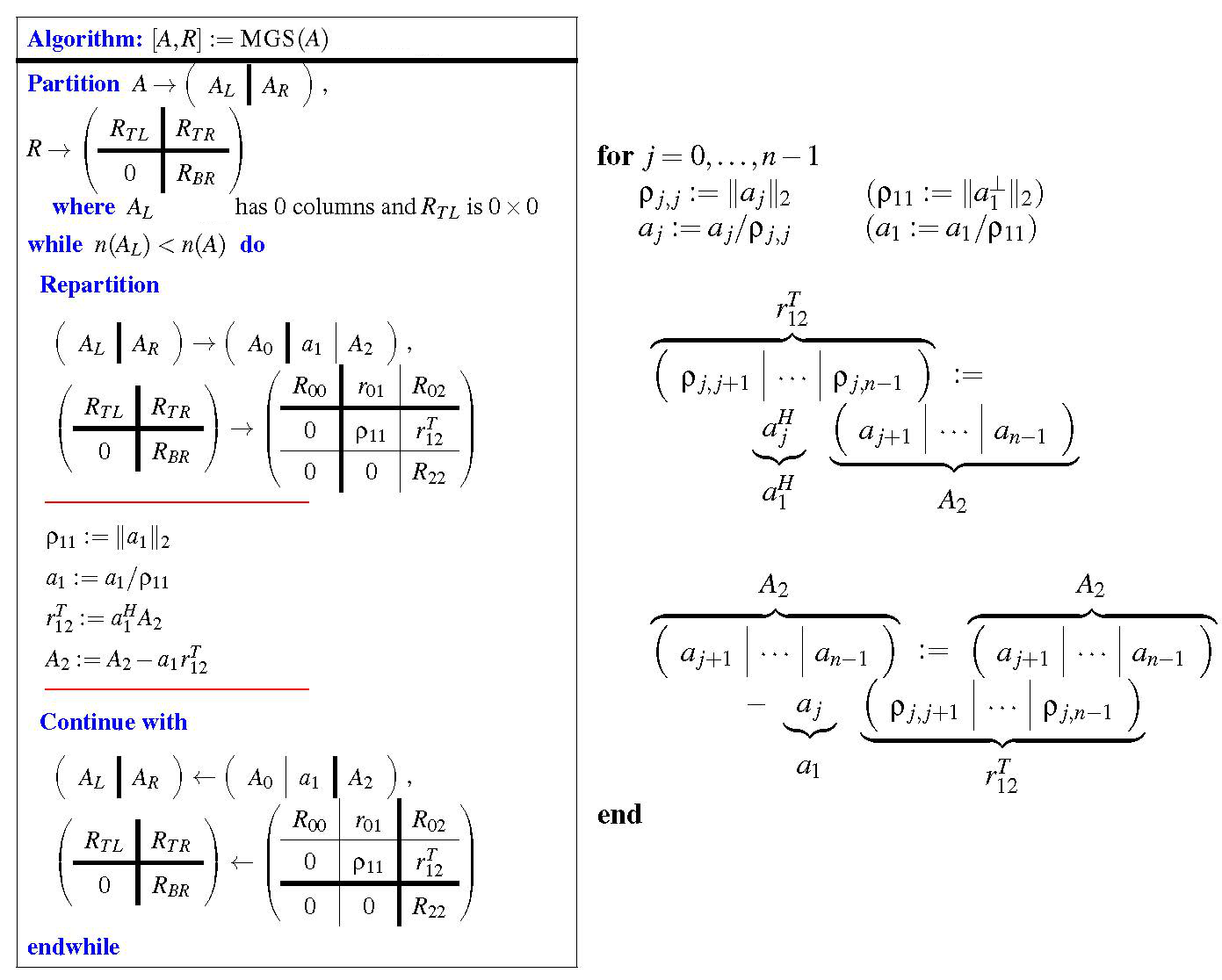
Gram-Schmidt process can be performed differently from CGS, and the corresponding algorithm is as follows, which is called Modified Gram-Schmidt (MGS) [3].
Consider $A=QR$.
Partition the given matrices as follows.
\[\left[\begin{array}{c|cc}A_{0} & a_{1} & A_{2}\end{array} \right]= \left[\begin{array}{c|cc}Q_{0} & q_{1} & Q_{2}\end{array} \right] \left[\begin{array}{c|cc} R_{0, 0} & r_{0, 1} & R_{0, 2} \\ \hline 0 & \rho_{1, 1} & r_{1, 2}^T\\ 0 & 0 & R_{2, 2} \end{array} \right]\]Assume that $a_1$ and $A_2$ are known.
Compute $\rho_{1,1}$ (compute the magnitude ↔︎ Step 2.).
- $\rho_{1,1}:=|a_1|$
Compute $q_1$ (compute the unit vector ↔︎ Step 3.).
- $q_1:=a_1/\rho_{1,1}$
Compute $r_{0,1}^T$, which is already known.
- $r_{0,1}^T:=q_1^H(A_2 - Q_2R_{22}) = q_1^HA_2$
Compute $A_2$ (update $A_2$ for the orthogonality ↔︎ Step 1.).
- $A_2:=A_2-q_1r_{0,1}^T$
Figure 2. shows Modified Gram-Schmidt algorithm for computing the QR factorization of a matrix A. The algorithm used FLAME notation.
Code 2. shows the algorithms in python language.
Code. 2: MGS QR in python
Why do we need this?
Through Gram-Schmidt process, we can obtain an orthonormal basis of the matrix $A$’s subspace, which has a set of lineary independent vectors {$a_0, …, a_{n-1}$}.
The advantages of being able to have an orthonormal basis are following [4].
- We can express any $v \in \mathbb{C}^n$ as a linear combination of coefficients, which will allows us to have an explicit formula expressing $v$ with the orthonormal basis.
- The explicit formula is very useful when dealing with projection onto subspace.
References
[1] M. M. Robert van de Geijn, “Advanced Linear Algebra: Foundations to Frontiers,” ALAFF Classical Gram-Schmidt (CGS). [Online]. Available: https://www.cs.utexas.edu/users/flame/laff/alaff/chapter03-classical-gram-schmidt.html. [Accessed: 03-Jan-2021].
[2] M. M. Robert van de Geijn, “Advanced Linear Algebra: Foundations to Frontiers,” ALAFF Classical Gram-Schmidt algorithm. [Online]. Available: https://www.cs.utexas.edu/users/flame/laff/alaff/chapter03-cgs-algorithm.html. [Accessed: 03-Jan-2021].
[3] M. M. Robert van de Geijn, “Advanced Linear Algebra: Foundations to Frontiers,” ALAFF Modified Gram-Schmidt (MGS). [Online]. Available: https://www.cs.utexas.edu/users/flame/laff/alaff/Modified-Classical-Gram-Schmidt.html. [Accessed: 03-Jan-2021].
[4] Michael Albanese, “Why is orthogonal basis important?,” Mathematics Stack Exchange. [Online]. Available: https://math.stackexchange.com/questions/518600/why-is-orthogonal-basis-important. [Accessed: 03-Jan-2021].