Speech Title: Grid-Aware Machine Learning for Distribution System Modeling, Monitoring, and Optimization
The contents covered in this article are credited to the speaker of the meeting, Dr. Zhu, and her research group members.
TL; DR
Speaker
- Shanny Lin
Abstract
Under limited obsevability conditions, the speaker presents approaches to modeling, monitoring, and optimization of distribution systems.
Keywords
- limited observability
- modeling
- linearized distribution model
- alternating minimization
- monitoring
- heterogeneous & dynamic data
- sptio-temporal learning
- optimization
- graph learning
- Conditional Value-at-Risk (CVaR)
Group Meeting Recap
Motivation
- Accurate network model is crucial for distributed energy resource (DER) monitoring and optimization.
- How to estimate an accurate model of the power system?
- How to address monitoring and optimization tasks under limited observability?
Problem Formulation
Modeling
- Linearized distribution flow model
- Difference between two consequtive time instance
- Estimate line parameter $\mathbf{\theta}$ bi-linear regression problem with Group-LASSO regularization
Monitoring
- DER visibility by leveraging heterogenous & dynamic data.
- Smart meter data ($\mathbf{\Gamma}$): lacks in time resolution
- D-PMU data ($\mathbf{Z}$): lacks in spatial diversity
- Smart meter data ($\mathbf{\Gamma}$): lacks in time resolution
- Active power matrix decompsition to low rank plus sparse model [2].
Optimization
- Optimal DER reactive power support problem
- DER optimization
- Fast-acting DER inverter control
Proposed Approach
Modeling
- Alternating Minimization (AM)
- Update $\mathbf{\theta}$ and ${\tilde{\mathbf{s}}^{\mathcal{u}}_{t}}$, alternatively.
Monitoring
- Spatio-temporal learning [1]
Optimization
- Graph learning
Experiment & Result
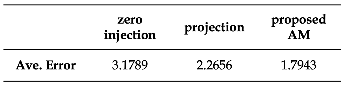
Modeling
- Experiment: Line reactance estimation
- Zero injection: $\tilde{\mathbf{s}}^{\mathcal{u}}_{t} = 0$.
- Projection: $\mathbf{P}(\tilde{\mathbf{v}}_t - \mathbf{A}(\tilde{\mathbf{s}}_t^o)\mathbf{\theta} - \mathbf{A}(\tilde{\mathbf{s}}_t^u)\mathbf{\theta} )$ such that $\mathbf{PA}(\tilde{\mathbf{s}}_t^u) = \mathbf{0}$.
- Alternating Minimization (AM)
- Zero injection: $\tilde{\mathbf{s}}^{\mathcal{u}}_{t} = 0$.
- Result
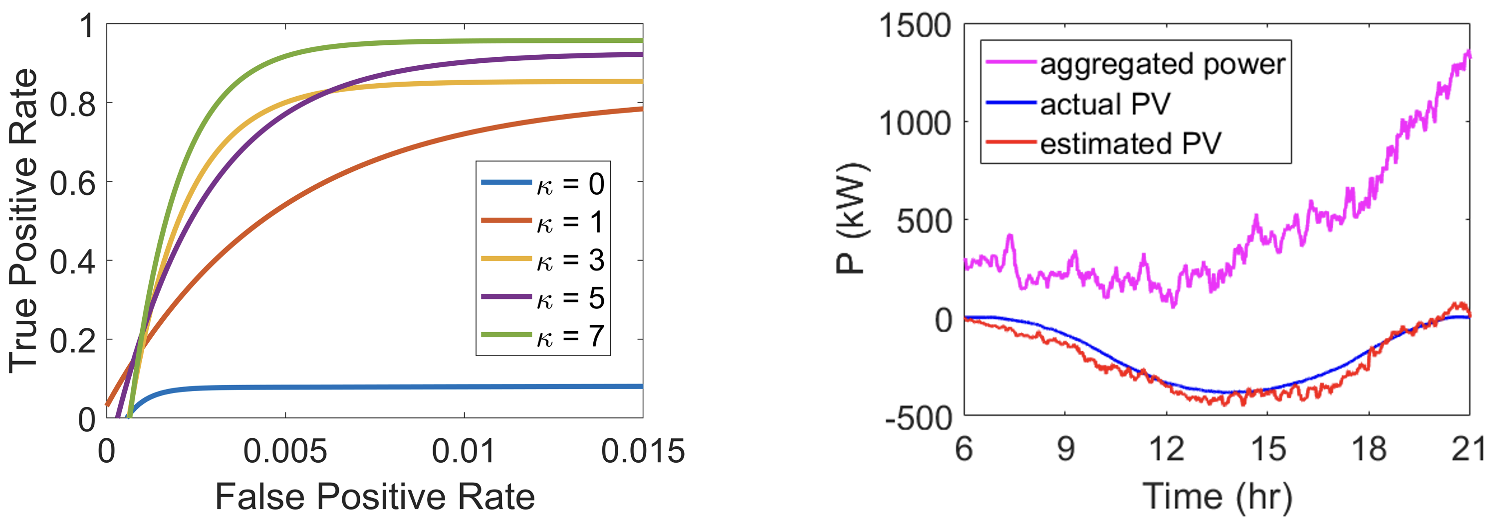
Monitoring
- Experiment: DER visibility by leveraging heterogeneous & dynamic data.
- Result
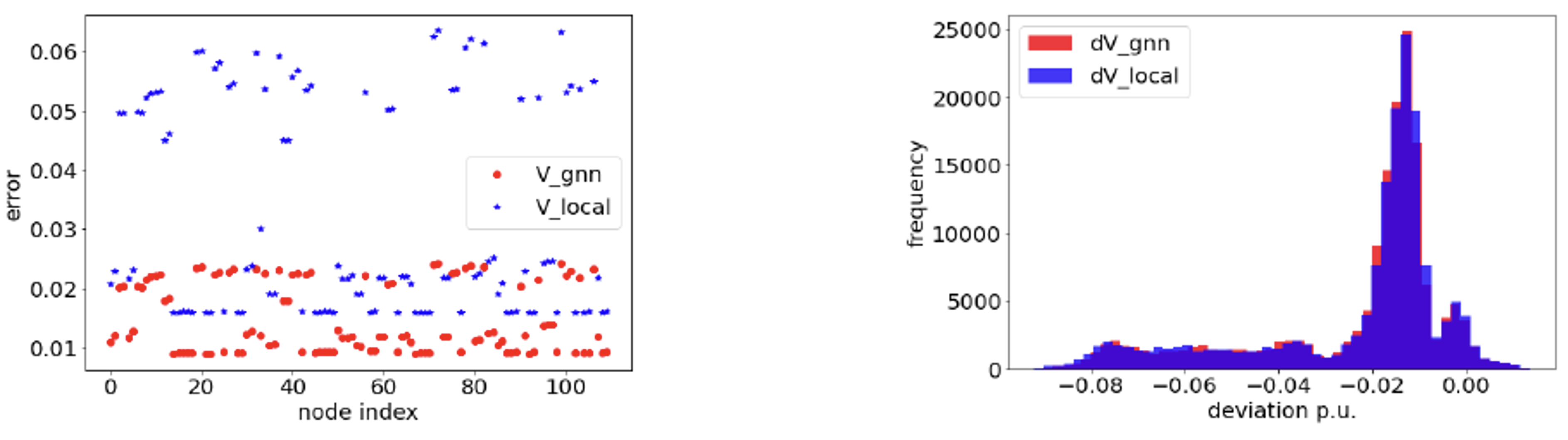
Optimization
- Experiment: Graph learning (w/o CVaR).
- Result
- Under voltage issue → it needs Conditional Value-at-Risk (CVaR).
Conclusion
- Modeling
- Estimated network line parameters under partial observability by solving a bi-linear regression problem by using AM algorithm.
- Estimated network line parameters under partial observability by solving a bi-linear regression problem by using AM algorithm.
- Monitoring
- Improved DER visibility by leveraging heterogeneous & dynamic data.
- Improved DER visibility by leveraging heterogeneous & dynamic data.
- Optimization
- Showed the need for CVaR method.
- Showed the need for CVaR method.
Future Study
- Online implementation for modeling.
- Online implementation for DER visibility.
- CVaR-aware GNN learning for DER optimization.
What I Benefit
Regularization [3]
Lasso and Ridge Regressions
Given a dataset ${X,y}$ where $X$ is the feature and $y$ is the label for regression, we simply model it as has a linear relationship $y = X\beta$. With regularization, we can control the degree of freedom of the model parameter ($\beta$) and able to avoid the risk of overfitting.
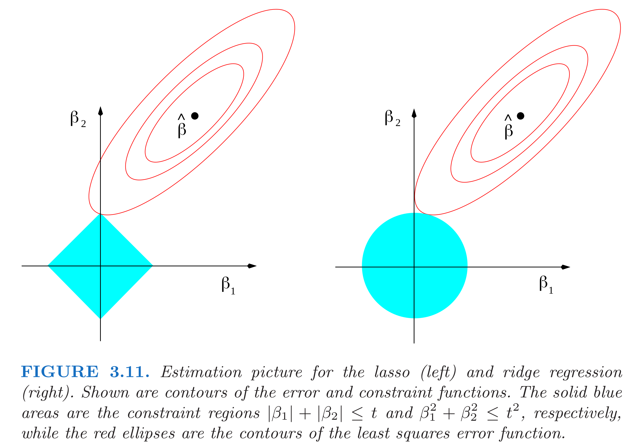
The two representative regularizations are LASSO (L1) and Ridge (L2), and they are defined as follows.
\[\beta^{*} = \underset{\beta}{\mathrm{argmin}} {\| y - X\beta \|_2^2} + \lambda \| \beta \|_{1}\] \[\beta^{*} = \underset{\beta}{\mathrm{argmin}} {\| y - X\beta \|_2^2} + \lambda \| \beta \|_{2}\]Due to the shape of their constraints boundary (norm ball shape), LASSO encourage a sparse result as a solution of the optimal problem.
Group LASSO
Suppose the weights in $\beta$ could be grouped, the new weight vector becomes $\beta_G = { \beta^{(1)}, \beta^{(2)},⋯,\beta^{(m)} }$. Each $\beta^{(l)}$ for $1 \leq l \leq m$ represents a group of weights from $\beta$.
We further group $X$ accordingly. We denote $X(l)$ as the submatrix of $X$ with columns corresponding to the weights in $\beta^{(l)}$. The optimization problem becomes
\[\beta^{*} = \underset{\beta}{\mathrm{argmin}} {\| y - \sum_{l=1}^{m}{X^{(l)}\beta^{(l)}} \|_2^2} + \lambda \sum_{l=1}^{m} \sqrt{p_{l}}\| \beta^{(l)} \|_{1}\]where $p_{l}$ represents the number of weights in $\beta^{(l)}$.
Why do we need GROUPING?
Usually, the variables of the minimization problem are not correlated. However, when there are certain constraints or correlations between variables, we need to group them appropriately.
The power injection as a minimization variable, covered in the presentation, is a good example. Since power is comprised of active and reactive power, the variable of the minimization problem of Eq. (3) has to be grouped as follows.
\[\tilde{\mathbf{s}}_{t} = \begin{bmatrix} \tilde{p}_n ; \tilde{q}_n \end{bmatrix}\]Risk management
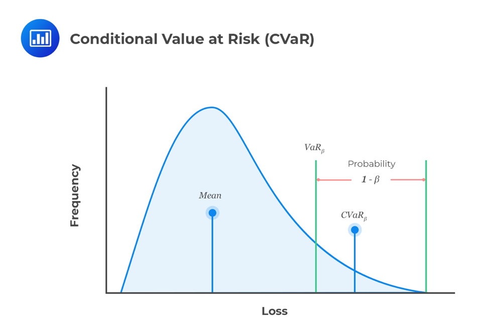
Value-at-Risk (VaR)
\[\begin{aligned} \int_{-\infty}^{VaR_{\beta}}&{f_{X}(x)}dx = 1 - \beta \\ & \text{where } f_{X}(x) \text{ is the marginal probability function of } X \\ & \text{and } \beta \in [0, 1] \text{ is the confidence level.} \end{aligned}\]or equivalently
\[P[x \geq VaR_{\beta}] = 1 - \beta\]Conditional Value-at-Risk (CVaR)
\[\begin{aligned} CVaR_{\beta} = & \frac{1}{1-\beta} \int_{-\infty}^{VaR_{\beta}}{x f_{X}(x)}dx \\ & \text{where } f_{X}(x) \text{ is the marginal probability function of } X \end{aligned}\]or equivalently
\[CVaR_{\beta} = E[x | x \geq VaR_{\beta}]\]The “CVaR at $(1-\beta)$% level” is the expected return on $X$ in the worst $(1-\beta)$% of cases. CVaR is an alternative to VaR that is more sensitive to the shape of the tail of the loss distribution [6].
What I Contribute
The framework of research/study
  1. Motivation
  2. Problem Formulation
  3. Proposed Approach
  4. Experiment & Result
  5. Future Study
The above list is the framework of research that Dr. Zhu discussed at the start of this year. Almost all research papers have been written along this process, which is also the basic step of our research.
However, it was not easy for me to summarize the contents of today’s meeting with this framework since there are three main topics in a single speech. Especially, it was hard to find the problem formulation part for monitoring. From my point of view, one of each topic is good enough for one individual presentation, and it would have been easier for me to fit the contents into this framework.
Therefore, I strongly suggest conducting our research and preparing our speech with this framework; then, it will help us draw better results in our research and deliver the main points more clearly to others.
Resting
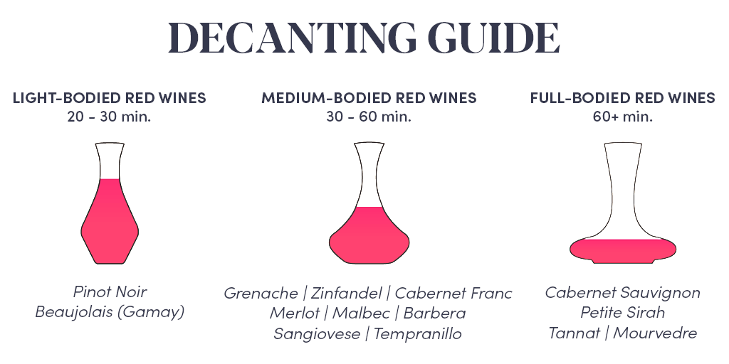
It is said that decanting is necessary to enjoy wine in its best quality. Likewise, our slides do want to have resting.
I think that taking some rest after writing (or making presentation slides) will introduce us to a higher level. To be more specific, it keeps us away from what we wrote and resets our minds, making us read more objectively.
For this reason, I suggest giving resting to your slides; then, it will allow you to have better results and makes you more confident in your speech.
References
[1]S. Lin and H. Zhu, “Enhancing the Spatio-temporal Observability of Grid-Edge Resources in Distribution Grids”, arXiv.org, 2021. [Online]. Available: https://arxiv.org/pdf/2102.07801.pdf. [Accessed: 18-Apr-2021].
[2]E. Candès, X. Li, Y. Ma and J. Wright, “Robust principal component analysis?”, Journal of the ACM, vol. 58, no. 3, pp. 1-37, 2011. Available: 10.1145/1970392.1970395 [Accessed: 17-Apr-2021].
[3]L. Mao, “Group Lasso,” Lei Mao’s Log Book. [Online]. Available: https://leimao.github.io/blog/Group-Lasso/. [Accessed: 17-Apr-2021].
[4]E. Golman, “The Ultimate Guide to Decanting & Aerating Kosher Wine,” Kosherwine.com, 18-Dec-2020. [Online]. Available: https://www.kosherwine.com/discover/the-ultimate-guide-to-decanting-kosher-wine. [Accessed: 17-Apr-2021].
[5]”Measuring and Modifying Risks. CFA Level 1 - AnalystPrep”, AnalystPrep. CFA® Exam Study Notes, 2021. [Online]. Available: https://analystprep.com/cfa-level-1-exam/portfolio-management/measuring-modifying-risks/. [Accessed: 17-Apr-2021].
[6]”Expected shortfall - Wikipedia”, En.wikipedia.org, 2021. [Online]. Available: https://en.wikipedia.org/wiki/Expected_shortfall. [Accessed: 17-Apr-2021].