This article is about a review of the paper [1], and is the second part of a personal research project to utilize the use of Graph Neural Network to the field of cascading outage prediction or detection.

I plan to utilize the model architecture used in this paper for cascading outage prediction.

• Research Project’s Git Repository

1. INTRODUCTION

1.1. What is the problem?

Transportation plays a vital role in everybody’s daily life. According to a survey in 2015, U.S. drivers spend about 48 minutes on average behind the wheel daily [2]. Under this circumstance, an accurate real-time forecast of traffic conditions is of paramount importance for road users, private sectors, and governments.

There were many efforts to monitor the current status of traffic conditions and to predict the future. These studies aimed to contribute to widely used transportation services, such as flow control, route planning, and navigation.

1.2. History of previous approaches

Previous studies on traffic prediction can be roughly divided into two categories: Dynamical modeling and Data-driven methods.

Many researchers are shifting their attention to data-driven approaches, since dynamical modeling methods have drawbacks as follow. 😡

• It requires sophisticated systematic programming.
  
  
• It consumes massive computational power.
  
  
• Impractical assumptions and simplifications among the modeling degrade the prediction accuracy.
  
  

As a result, Deep learning approaches, which are major representatives of data-driven approaches, have been widely and successfully applied to various traffic tasks. Significant progress has been made in following works. 😁

• Deep belief network (DBN) [3]
  
  
• Stacked auto-encoder (SAE) [4]
  
  

However, it is difficult for these dense networks to extract spatial and temporal features from the input jointly. 😡

To take full advantage of spatial features, some researchers use convolutional neural network (CNN) to capture adjacent relations among the traffic network, along with employing recurrent neural network (RNN) on time axis. 😁

However, this approach has limitations as follow. 😡

• The normal convolutional operation applied restricts the model to only process grid structures (e.g. images, videos) rather than general domains.
  
  
• Rrecurrent networks for sequence learning require iterative training, which introduces error accumulation by steps.
  
  
• RNN-based networks are widely known to be difficult to train and computationally heavy.

1.3. Proposed Approach

For overcoming the limitations of previous approaches, the author introduces several strategies to effectively model temporal dynamics and spatial dependencies of traffic flow. 😁

• To fully utilize spatial information, the author models the traffic network by a general graph instead of treating it separately (e.g. grids or segments).
  
  
• To handle the inherent deficiencies of recurrent networks, the author employs a fully convolutional structure on time axis.
  
  

Above all, the author proposes a novel deep learning architecture, the spatio-temporal graph convolutional networks (STGCN), for traffic forecasting tasks. 🤘

Q. IS THERE ANY DRAWBACK IN STGCN???
A.

2. PRELIMINARY

2.1. Traffic Prediction on Road Graphs

Traffic forecast as a typical time-series prediction problem

Predicting the most likely traffic measurements (e.g. speed or traffic flow) in the next $H$ time steps given the previous $M$ traffic observations as,

where $v_t \in \mathbb{R}^{n}$ is an observation vector of $n$ road segments at time step $t$, each element of which records historical observation for a single road segment.

Graph structured traffic time series problem

In this work, the author defines the traffic network on a graph and focuses on structured traffic time series. The traffic network is represented as an undirected graph (or directed one) $\mathcal{G_t}$ with weights $w_{ij}$ as shown in Figure 1.

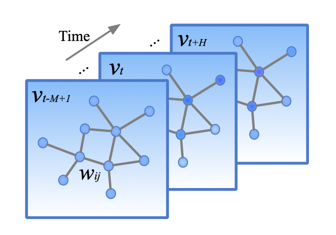
At the $t$-th time step, in graph $\mathcal{G}_t = (\mathcal{V}_t, \mathcal{E}, W)$,

• $\mathcal{V}_t$ is a finite set of vertices, corresponding to the observations from $n$ monitor stations at time $t$.
  
  
• $\mathcal{E}$ is a set of edges, indicating the connectedness between stations.
  
  
• $W \in \mathbb{R}^{n \times n}$ denotes the weighted adgacency matrix of $\mathcal{G}_t$.
  
  

Q. DOES EDGES CAN HAVE ITS OWN TIME VARIANT VARIABLES???
  (e.g. temperature of transmission lines in power system)
A.

2.2. Convolutions on Graphs

In this paper, the author introduces the notion of graph convolution operator “$*\mathcal{G}$” based on the conception of spectral filtering [7, 8].

where

• $x \in \mathbb{R}^{n}$ is a graph signal as an input (data from each vertex).
  
  
• $y \in \mathbb{R}^{n}$ is filtered signal as an output.
  
  
• $\Theta(\cdot)$ is a kernel (characteristic of the filter).
  
  
• $U = [u_0, …, u_{n-1}] \in \mathbb{R}^{n\times n}$, Graph Fourier basis, is the matrix of eigenvectors of the normalized graph Laplacian $L$.
  
  
• $\Lambda =diag([\lambda_0, …, \lambda_{n-1}]) \in \mathbb{R}^{n\times n}$ is the matrix of eigenvalues of the normalized graph Laplacian $L$.
  
  (check details of Laplacian matrix in appendix 7.1)

As a result, a graph signal $x$ is filtered by a kernel $\Theta$ can be defined with multiplication between $\Theta$ and graph Fourier transform $U^T x$ [7].

(check details of graph Fourier transform in appendix 7.2)

In addition, due to its matrix multiplication, the computational complexity of graph convolution is $\mathcal{O}(n^2)$.

Q. WHY “NORMALIZED” L???
A.

3. PROPOSED MODEL

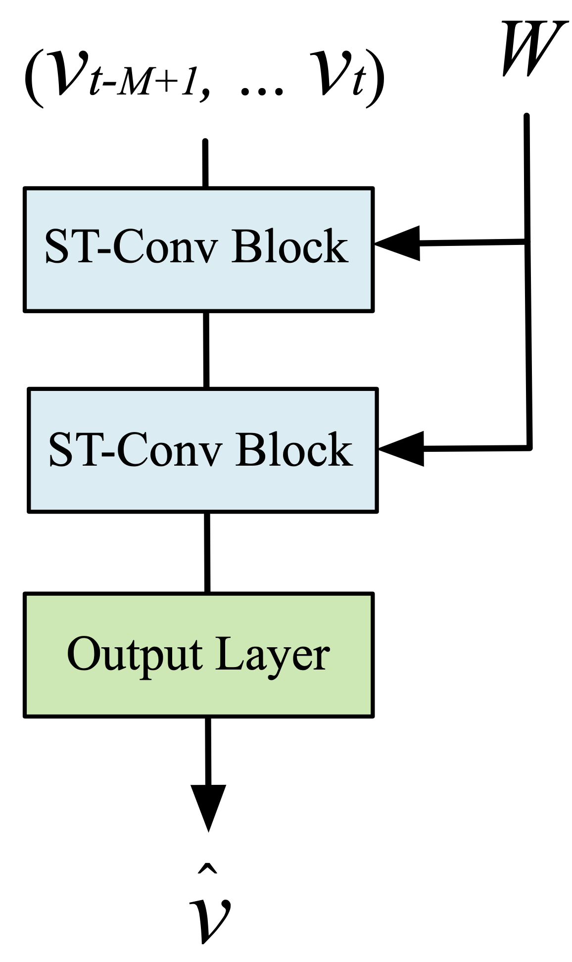
3.1. Network Architecture

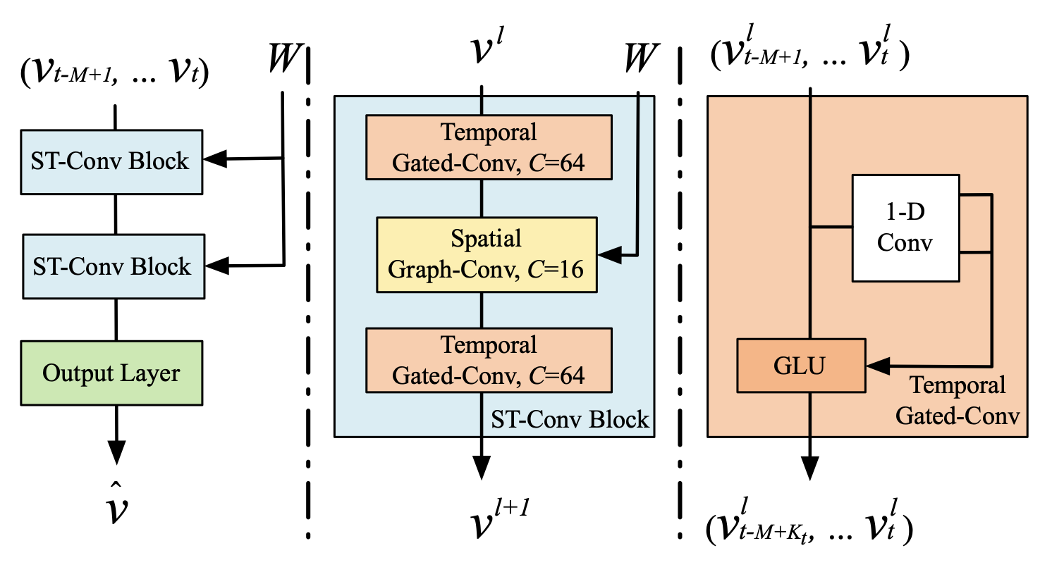
The author proposed a model architecture called spatio-temporal graph convolutional networks (STGCN). As shown in Figure 2, STGCN is composed of several spatio-temporal convolutional blocks. Each spatio-temporal convolutional blocks is formed as a “sandwich” structure with two gated sequential convolution layers and one spatial graph convolution layer in between.

3.2. Graphs CNNs for Extracting Spatial Features

The traffic network generally organizes as a graph structure. Since 2-D convolutions on grids can only capture the spatial locality, attributes of traffic networks (graph structured data) were not fully extracted by 2-D convolution filters.

Accordingly, in STGCN, the graph convolution is employed directly on graph-structured data to extract highly meaningful patterns and features in the space domain.

However, there are two issues of the graph convolution expressed in Eq. (2). 😡

• The kernel is not localized in space yet.
  
  
• The computation of kernel $\Theta$ in graph convolution by Eq. (2) can be expensive due to $\mathcal{O}(n^2)$ multiplications with graph Fourier basis.
  
  

The authors applied two approximation strategies to overcome these issues. 😁

Chebyshev Polynomials Approximation

Chebyshev polynomial $T_k(x)$ is used to approximate kernels as a truncated expansion of order $K-1$ as follows.

where

• $\tilde{\Lambda} = 2 \frac{\Lambda}{\lambda_{max}}-I_n$ ($\lambda_{max}$ denotes the largest eigenvalues of $L$).
  
  
• $\theta \in \mathbb{R}^{n}$ is a vector of polynomial coefficient.
  
  (check details of Chebyshev polynomials approximation in appendix 7.3)

Using the Chebyshev polynomials approximation, the graph convolution can then be rewritten as,

where

• $T_k(\tilde{L})\in\mathbb{R}^{n\times n}$ is the Chebyshev polynomial of order $k$
  
  
• $\tilde{L} \in \mathbb{R}^{n \times n}$ the scaled Laplacian $\tilde{L} = 2\frac{L}{\lambda_{max}} - I_n$.
  
  

As a result, we can localize the filter by restricting kernel $\Theta$ to a polynomial of order $k$.

Moreover, by recursively computing $K$ convolutions through the polynomial approximation, the cost of Eq. (2) can be reduced to $\mathcal{O}(K|\mathcal{E}|)$ as Eq. (3) shows [8].

(check details of localizing convolution filters in appendix 7.4)

Q. RESCALED??? WHY???
A. It makes eigenvalues in the range [-1, 1] to prepare for the recursive computation.

Q. WHY |E| IN COMPUTAIONAL COMPLEXITY???
A.

1st-order Approximation

A layer-wise linear formulation can be defined by stacking multiple localized graph convolutional layers with the first-order approximation of graph Laplacian [9].

Due to the scaling and normalization in neural networks, we can further assume that $\lambda_{max} \approx 2$.

Q. THE SCALING AND NORMALIZATION IN NEURAL NETS???
A.

Thus, the Eq. (3) can be simplified to,

where $\theta_0$, $\theta_1$ are two shared parameters of the kernel.

In order to constrain parameters and stabilize numerical performances, $\theta_0$ and $\theta_1$ are replaced by a single parameter $\theta$ by letting $\theta = \theta_0 = -\theta_1$.

Then, the graph convolution can be alternatively expressed as,

where

• $W$ is renormalized by $\tilde{W} = W + I_n$
  
  
• $D$ is renormalized by $\tilde{D_{ii}} = \sum_j{\tilde{W}_{ij}}$.
  
  

The authors stack the 1st-order approximation $K$ layers vertically. In this scenario, $K$ is the number of successive filtering operations, and the stack achieves the similar effect as $K$-localized convolutions do horizontally.

Additionally, the layer-wise linear structure is parameter-economic and highly efficient for large-scale graphs, since the order of the approximation is limited to one.

(check details of localizing convolution filters in appendix 7.4)

Generalization of Graph Convolutions

The graph convolution operator “$*\mathcal{G}$” defined on $x \in \mathbb{R}^n$ can be extended to multi-dimensional tensors.

For a signal $C_i$ channels $X \in \mathbb{R}^{n \times C_i}$, the graph convolution can be generalized by,

with the $C_i \times C_o$ vectors of Chebyshev coefficients $\Theta_{ij} \in \mathbb{R}^K$ ($C_i$, $C_o$ are the size of input and output of the feature maps, respectively).

The graph convolution for 2-D variables is denoted as “$\Theta *\mathcal{G}X$” with $\Theta \in \mathbb{R}^{K \times C_i \times C_o}$.

3.3. Gated CNNs for Extracting Temporal Features

RNNs for traffic prediction still suffer from following. 😡

• time-consuming iterations
  
  
• complex gate mechanisms
  
  
• slow response to dynamic changes.
  
  

On the contrary, CNNs have the superiority as follows. 😁

• fast training
  
  
• simple structures
  
  
• no dependency constraints to previous steps.
  
  

The authors employ entire convolutional structures on time axis to capture temporal dynamic behaviors of traffic flows.

This specific design allows parallel and controllable training procedures through multi-layer convolutional structures formed as hierarchical representations.

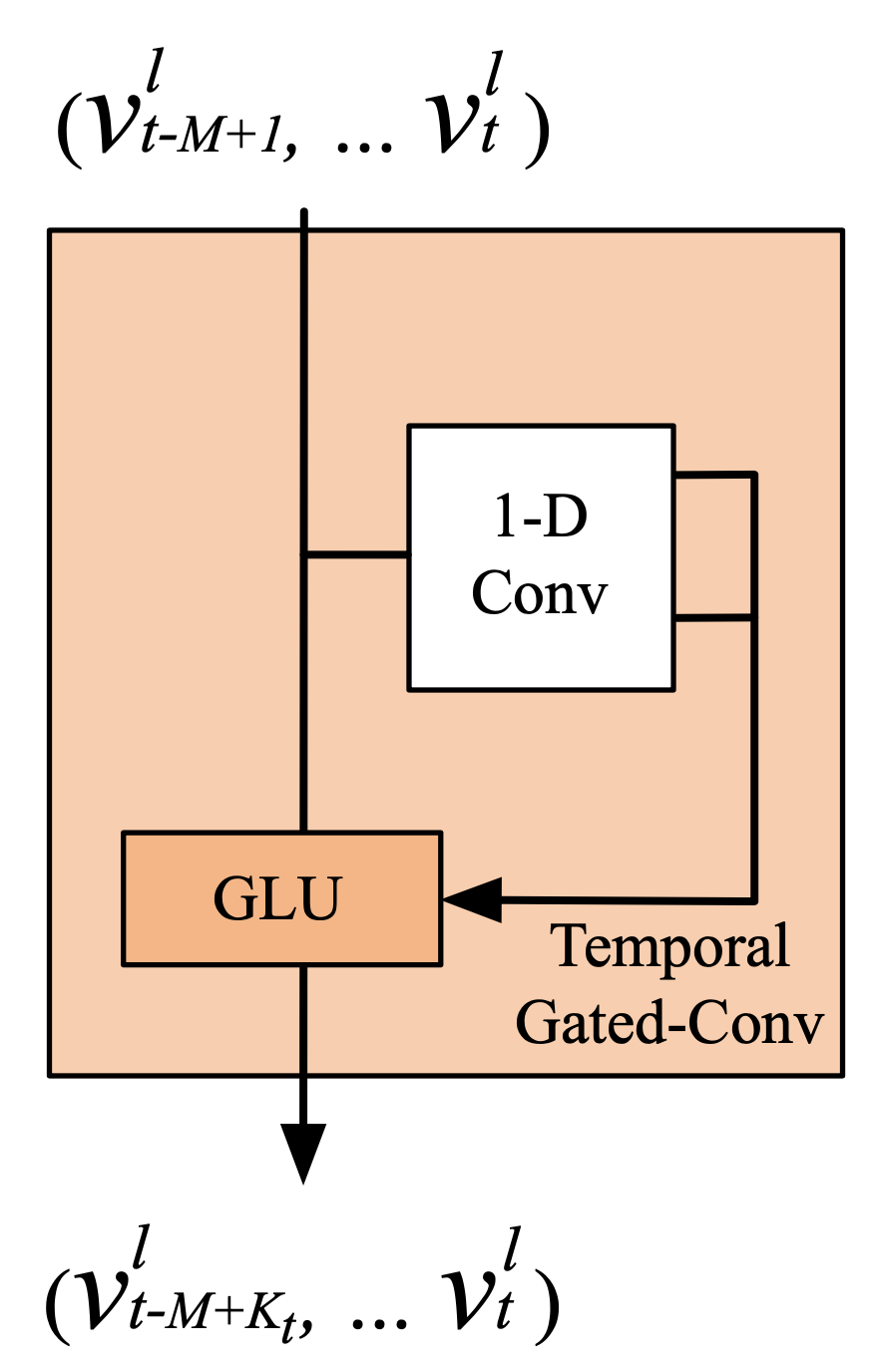
For each node in graph $\mathcal{G}$, the temporal convolution explores $K_t$ neighbors of input elements without padding which leading to shorten the length of sequences by $K_{t}-1$ each time. Thus, input of temporal convolution for each node can be regarded as a length-$M$ sequence with $C_i$ channels as $Y \in \mathbb{R}^{M \times C_i}$.

The convolution kernel $\Gamma \in \mathbb{R}^{K_t \times C_i \times 2C_o}$ is designed to map the input $Y$ to a single output element $[P : Q] \in \mathbb{R}^{(M-K_t+1) \times (2C_o)}$ ($P, Q$ is split in half with the same size of channels).

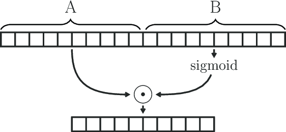
As a result, the temporal gated convolution can be defined as,

where

• $P, Q$ are input of gates in GLU respectively
  
  
• $\odot$ denotes the element-wise Hadamard product.
  
  
• $\sigma$ is sigmoid gate controls which input $P$ of the current states are relevant for discovering compositional structure and dynamic variances in time series.
  
  

Q. WHY GLU, NOT ReLU OR SOMETHING ELSE???
A.

The non-linearity gates contribute to the exploiting of the full input filed through stacked temporal layers as well. Furthermore, residual connections are implemented among stacked temporal convolutional layers. Similarly, the temporal convolution can also be generalized to 3-D variables by employing the same convolution kernel $\Gamma$ to every node $\mathcal{Y}_i \in \mathbb{R}^{M \times C_i}$ (e.g. sensor stations) in $\mathcal{G}$ equally, noted as “$\Gamma * \tau \mathcal{Y}$” with $\mathcal{Y} \in \mathbb{R}^{M \times n \times C_i}$.

3.4. Spatio-Temporal Convolutional Block

In order to fuse features from both spatial and temporal domains, the spatio-temporal convolutional block (ST-Conv block) is constructed to jointly process graph-structured time series.

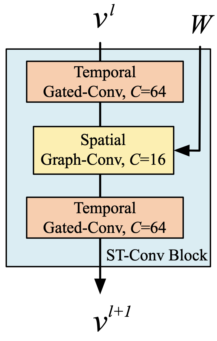
As illustrated in Figure 5, the spatial layer in the middle is to bridge two temporal layers which can achieve fast spatial-state propagation from graph convolution through temporal convolutions.

The “sandwich” structure also helps the network sufficiently apply bottleneck strategy to achieve scale compression and feature squeezing by downscaling and upscaling of channels $C$ through the graph convolutional layer.

Q. WHY IT HAS SANDWICH STRUCTURE???
A.

Moreover, layer normalization is utilized within every ST-Conv block to prevent overfitting.

The input and output of ST-Conv blocks are all 3-D tensors. For the input $v^l \in \mathbb{R}^{M \times n \times C^l}$ of block $l$, the output $v^{l+1} \in \mathbb{R}^{(M-2(K_t-1)) \times n \times C^{l+1}}$is computed by,

where

• $\Gamma_0^l$, $\Gamma_1^l$ are the upper and lower temporal kernel within block $l$, respectively.
  
  
• $\Theta^l$ is the spectral kernel of graph convolution
  
  
• $ReLU(\cdot)$ denotes the rectified linear units function.
  
  

3.5. Loss Function

We use L2 loss to measure the performance of our model.

where

• $W_\theta$ are all trainable parameters in the model
  
  
• $v_{t+1}$ is the ground truth
  
  
• $\hat{v}(\cdot)$ denotes the model’s prediction
  
  

3.6. Recap of the Main Characteristics STGCN

• STGCN is a universal framework to process structured time series.
  
  
• It is not only able to tackle traffic network modeling and prediction issues but also to be applied to more general spatio-temporal sequence learning tasks.
  
  
• The spatio-temporal block combines graph convolutions and gated temporal convolutions, which can extract the most useful spatial features and capture the most essential temporal features coherently.
  
  
• The model is entirely composed of convolutional structures and therefore achieves parallelization over input with fewer parameters and faster training speed.
  
  

4. EXPERIMENTS & RESULTS

4.1. Dataset Description

BJER4 was gathered from the major areas of east ring No.4 routes in Beijing City by double-loop detectors.

• The traffic data are aggregated every 5 minutes.
  
  
• There are 12 roads selected for the experiment.
  
  

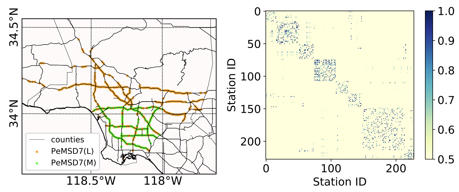
PeMSD7 was collected from Caltrans Performance Measurement System (PeMS) in real-time by over 39,000 sensor stations, deployed across the major metropolitan areas of California state highway system.

• The traffic data are aggregated every 5 minutes.
  
  
• The authors randomly select a medium and a large scale among the District 7 of California containing 228 and 1,026 stations, labeled as PeMSD7(M) and PeMSD7(L), respectively, as data sources (shown in the left of Figure 7).
  
  

4.2. Data Preprocessing

• Interpolation method: Linear interpolation
  
  
• Normalization method: Z-score
  
  

4.3. Experimental Settings

All the tests use 60 minutes as the historical time window.

With Eq. (1) and the time window setting, 12 observed data points ($M = 12$) are used to forecast traffic conditions in the next 15, 30, and 45 minutes ($H = 3, 6, 9$).

Evaluation Metric

To measure and evaluate the performance of different methods, three following metrics are adopted.

• Mean Absolute Errors (MAE)

• Mean Absolute Percentage Errors (MAPE)

• Root Mean Squared Errors (RMSE)

Q. WHY DO WE NEED MULTIPLE METRICS???
A.

Baselines

The authors set up two types of models based on STGCN framework.

• STGCN(Cheb) with the Chebyshev polynomials approximation
  
  
• STGCN(1st) with the 1st-order approximation ($K=1$).
  
  

STGCN based models are compared with following baselines.

• Historical Average (HA)
  
  
• Linear Support Vector Regression (LSVR)
  
  
• Auto-Regressive Integrated Moving Average (ARIMA)
  
  
• Feed-Forward Neural Network (FNN)
  
  
• Full-Connected LSTM (FC-LSTM)
  
  
• Graph Convolutional GRU (GCGRU)
  
  

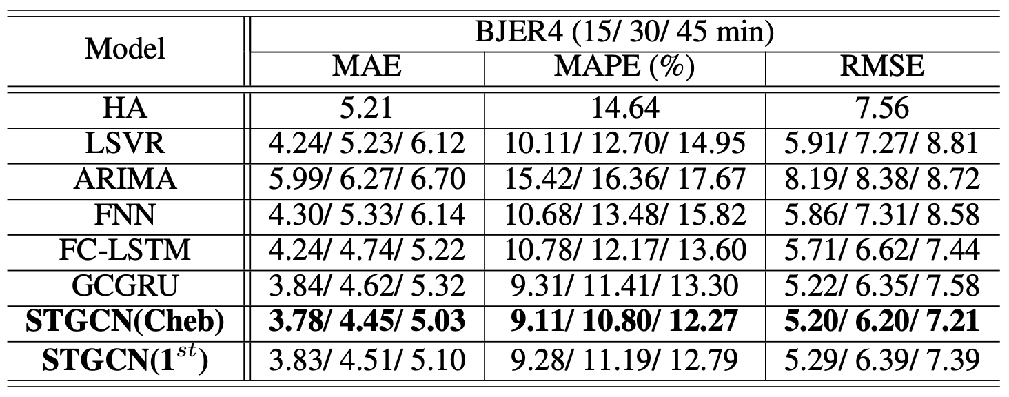
4.4. Experimental Results

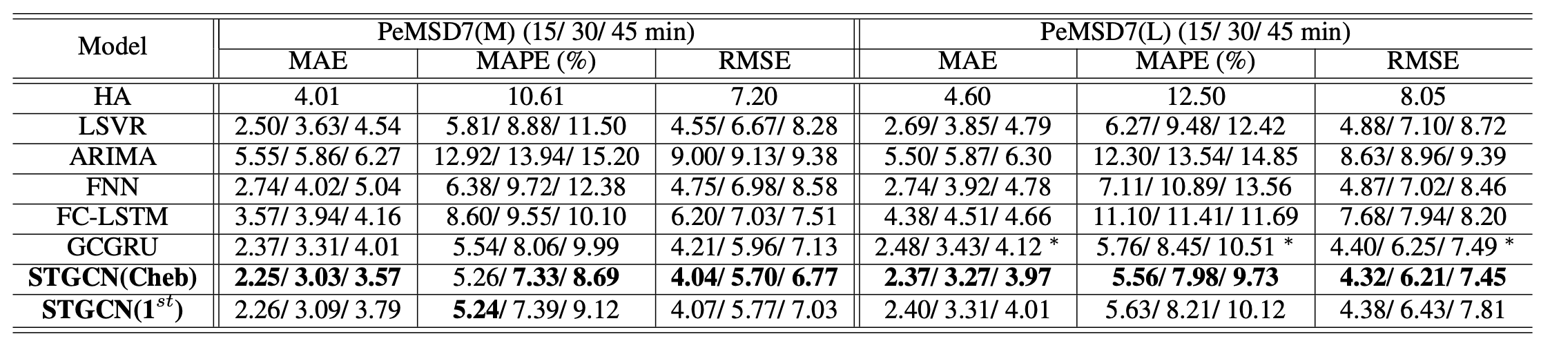
Benefits of Spatial Topology

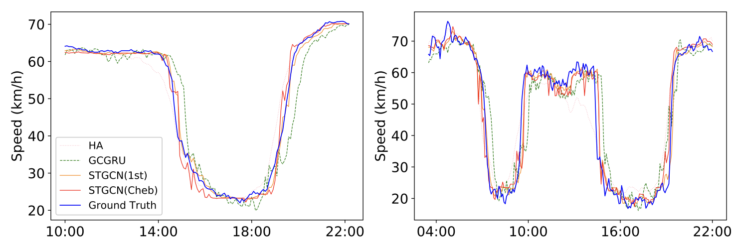
Through effectively utlizing spatial structure of the given data, the STGCN based models have achieved a significant improvement on short and mid-and-long term forecasting.

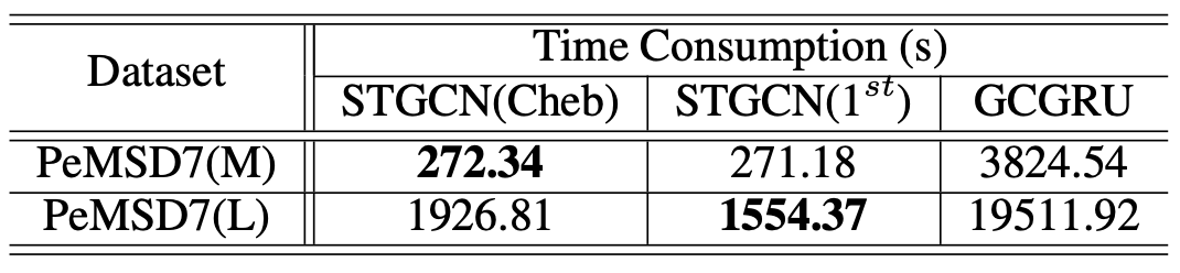
Training Efficiency and Generalization

To see the benefits of the convolution along time axis in our proposal, we summarize the comparison of training time between STGCN and GCGRU in Table 3.

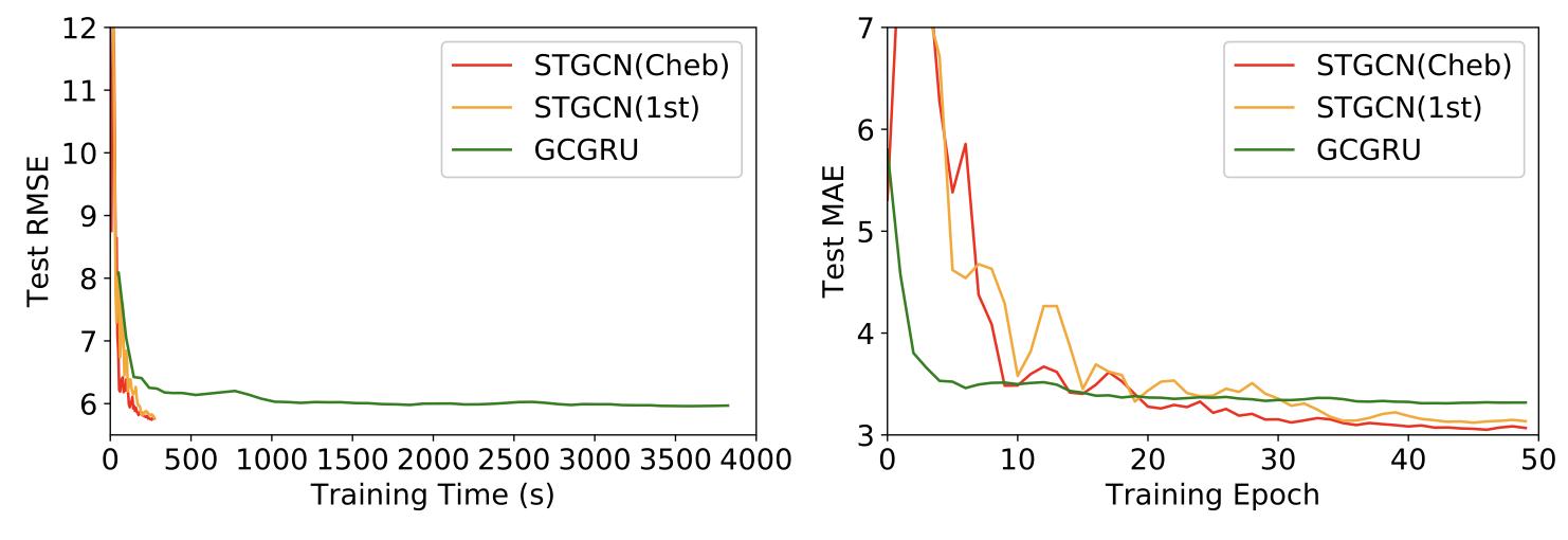
In order to further investigate the performance of compared deep learning models, the authors plot the RMSE and MAE of the test set of PeMSD7(M) during the training process, see Figure 9.

Those figures also suggest that the models can achieve muchfaster training procedure and easier convergences. Thanks to the special designs in ST-Conv blocks, the models have superior performances in balancing time consumption and parameter settings.

Q. HOW IT ACHIEVES SUPERIOR PERFORMANCE IN BALANCING TIME COMSUMPTION & PARAMETER SETTING???
A.

Moreover, the number of parameters in STGCN ($4.54 \times 10^5$) only accounts for around two third of GCGRU, and saving over 95% parameters compared to FC-LSTM.

5. CONCLUSION

In this paper, the authors propose

• A novel deep learning framework STGCN for traffic prediction.
  
  
• Integrating graph convolution and gated temporal convolution through spatio-temporal convolutional blocks.
  
  

The experiments shows

• Benefits of spatial topology
  
  
  • The model outperforms other state-of-the-art methods on two real-world datasets.
    
    
  • The results indicate its great potentials on exploring spatio-temporal structures from the input.
    
    
• Training efficiency and generalization
  
  
  • Faster training (parallelization).
    
    
  • Fewer parameters with flexibility and scalability.
    
    

Q. WHY/HOW IT ACHEIVES FELXIBILITY AND SCALABILITY???
A.

These features are quite promising and practical for scholarly development and large-scale industry deployment. In the future, we will further optimize the network structure and parameter settings.

Moreover, the proposed framework can be applied into more general spatio-temporal structured sequence forecasting scenarios, such as evolving of social networks, and preference prediction in recommendation systems, etc.

6. MY RESEARCH PROJECT

Purpose / Goal

• Forecast or detect (in real-time) cascading outages in power systems.

Approach

• Use a GNN based model to predict or detect cascading outages.

Experiments

Step 1. Data Generation

• Need to introduce randomness to create large size of dataset.
  
  

• Randomness will be given by the method that generated the uncertain loads in [16]:
  
  

  \[d := d + \mathcal{N}(\mu=0, \sigma = 0.03 * d)\]
  • $d$ is a load.
    
    
  • $\mathcal{N}$ is normal distribution with mean zero and standard deviation proportional to the load.
    
    

Q. WHICH FEATURES (e.g. $P_d, Q_d, P_g, Q_g$ or outage event time $t_{event}$) SHOULD BE GIVEN RANDOMNESS?
A.

• Codes
  
  
  • Generate N-2 Contingency Datasets.py
    
    
  • Generate Datasets.ipynb
    
    
  • Exploratory Data Analysis.ipynb
    
    

Step 2. Design the GNN Model Architecture

• The model should able to utilze spatial and temporal feature of the data.
  
  
  • graph structured data: spatial feature
    
    
  • time series data: temporal feature
    
    
• Models based on STGCN architecture [1] can extract and learn the both features (spatial & temporal) from the data.
  
  

• Codes
  
  
  • yet not ready…😭
    
    

Step 3. Train & Test the Model

• 🤔

Step 4. Tune the Hyper-parameters

• 🤔

Results (What we want to see…)

• High enough prediction (or detection) accuracy.
  
  
• Extremely high computational efficiency compared to old methods.
  
  
• A GNN based model having significantly fewer nodes (trainable parameters) than other deep learning models.
  
  

7. APPENDIX

7.1. Laplacian & Symmetric normalized Laplacian [10]

Laplacian

Given a simple graph $\mathcal{G}$ with $n$ vertices, its Laplacian matrix $L_{n \times n}$ is defined as,

where

• $D$ is the degree matrix of the graph.
  
  
• $A$ is adjacency matrix.
  
  

The elements of $L$ are given by

where

• $deg(v_i)$ is the degree of the vertex $i$.

Symmetric normalized Laplacian

The symmetric normalized Laplacian matrix is defined as,

The elements of $L^{sym}$ are given by

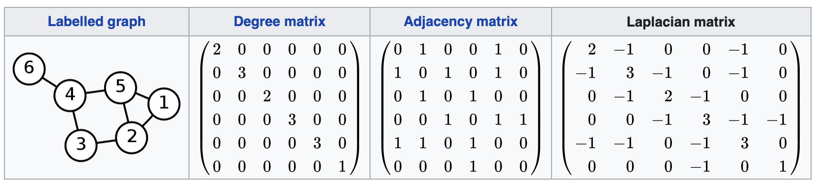
7.2. Graph Fourier transform

Graph Fourier transform is a mathematical transform which eigendecomposes the Laplacian matrix of a graph into eigenvalues and eigenvectors. Analogously to classical Fourier Transform, the eigenvalues represent frequencies and eigenvectors form what is known as a graph Fourier basis [11].

Lets assume we have a graph $\mathcal{G}_t = (\mathcal{V}, \mathcal{E}, W)$, where $\mathcal{V}$ is a finite set of $|\mathcal{V}|=n$ verices, $\mathcal{E}$ is a set of edges, and $W \in \mathbb{R}^{n\times n}$ is a weighted adjacency matrix.

The definition of Laplacian matrix is

where

• $I_n$ is an identity matrix.
  
  
• $D \in \mathbb{R}^{n\times n}$ is the diagonal degree matrix with $D_{ii} = \sum_{j}{W_{ij}}$.
  
  
• $U = [u_0, …, u_{n-1}] \in \mathbb{R}^{n\times n}$ is a Graph Fourier basis.
  
  
• $\Lambda =diag([\lambda_0, …, \lambda_{n-1}]) \in \mathbb{R}^{n\times n}$ is the diagonal matrix of eigenvalues of $L$.
  
  

The graph Fourier transform of a signal $x \in \mathbb{R}^{n}$ is then deinfed as as $\hat{x} = U^{T}x \in \mathbb{R}^{n}$, and its inverse as $x=U\hat{x}$ [13].

7.3. Chebyshev Polynomial & Approximation [14, 15]

The Chebyshev polynomials are two sequences of polynomials related to the sine and cosine functions, notated as $T_n(x)$ and $U_n(x)$.

The Chebyshev polynomials of the first kind are obtained from the recurrence relation as follows.

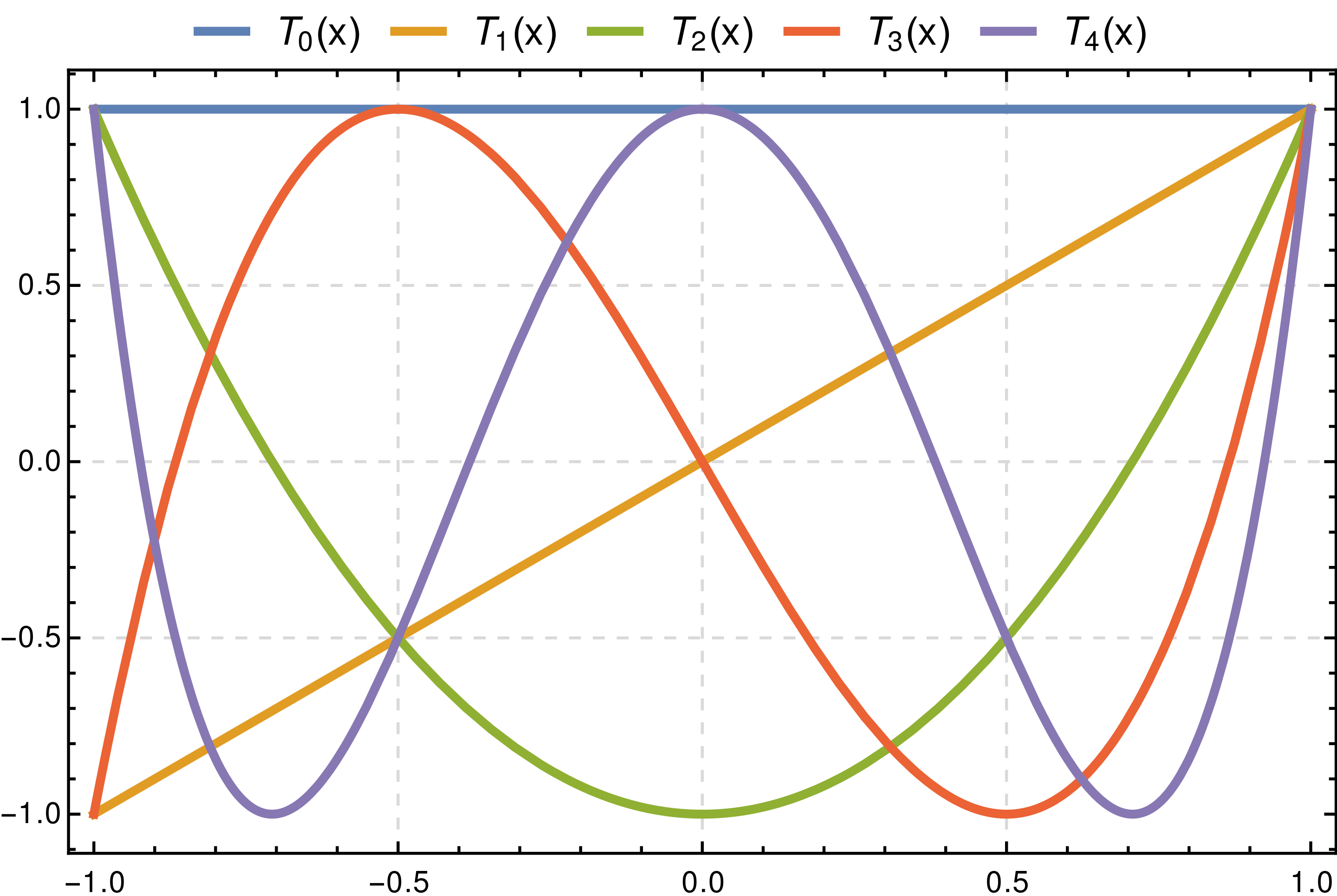
One can obtain polynomials very close to the optimal one by expanding the given function in terms of Chebyshev polynomials and then cutting off the expansion at the desired degree.

This is similar to the Fourier analysis of the function, using the Chebyshev polynomials instead of the usual trigonometric functions.

7.4. Localizing Convolutional Filter in Space

The Eq. (2) represents spectral filtering of graph signal.

The filter is characterized by its kernel ($\Theta(\cdot)$), and the simplest kernerl we can imagine is a non-parametic filter, i.e. the kernel parameters $\theta_k \in \mathbb{R}$ $(k=1, …, n)$ are all free.

In this case, the filter has a limitaion that it is not localized in space. 😡

However, this issue can be solved by following two strategies. 😁

A. Restricting kernel to polynomial by Chebyshev approximation (Horizontal ver.)

We can localize the filter in space by restricting the kernel to a polynomial [8]. As a result, the convolutional filter is restricted as a polynomial filter. Moreover, by using Chebyshev approximation, we could limit the radius of the convolutional operation.

The localized filter can be expressed as follows.

where

• $\tilde{\Lambda} = 2 \frac{\Lambda}{\lambda_{max}}-I_n$ ($\lambda_{max}$ denotes the largest eigenvalues of $L$).
  
  
• $\theta \in \mathbb{R}^{n}$ is a vector of polynomial coefficient.
  
  
• $K$ is a radius of the convolutional filter.
  
  

B. Applying a stack of 1st-order approximated kernel (Vertical ver.)

By 1st-order approximation, we can get a simplified filter as follows.

where $\theta_0$, $\theta_1$ are two shared parameters of the kernel.

Applying a stack of graph convolutions with the 1st-order approximation vertically that achieves the similar effect as $K$-localized convolutions do horizontally, all of which exploit the information from the $(K-1)$-order neighborhood of central nodes [1].

Reference

[1] B. Yu, H. Yin, and Z. Zhu, “Spatio-Temporal Graph Convolutional Networks: A Deep Learning Framework for Traffic Forecasting,” arXiv.org, 12-Jul-2018.

[2] B. Tefft, S. Rosenbloom, R. Santos, and T. Triplett, “American Driving Survey: 2014 – 2015,” AAA Foundation, 14-Jun-2018. [Online]. Available: https://aaafoundation.org/american-driving-survey-2014-2015/. [Accessed: 15-Feb-2021].

[3] Yuhan Jia, Jianping Wu, and Yiman Du, “Traffic speed prediction using deep learning method,” 2016 IEEE 19th International Conference on Intelligent Transportation Systems (ITSC), 2016.

[4] Y. Lv, Y. Duan, W. Kang, Z. Li and F. Wang, “Traffic Flow Prediction With Big Data: A Deep Learning Approach,” in IEEE Transactions on Intelligent Transportation Systems, vol. 16, no. 2, pp. 865-873, April 2015, doi: 10.1109/TITS.2014.2345663.

[5] M. Niepert, M. Ahmed, and K. Kutzkov, “Learning Convolutional Neural Networks for Graphs,” arXiv.org, 08-Jun-2016. [Online]. Available: https://arxiv.org/abs/1605.05273. [Accessed: 05-Apr-2021].

[6] J. Bruna, W. Zaremba, A. Szlam, and Y. LeCun, “Spectral Networks and Locally Connected Networks on Graphs,” arXiv.org, 21-May-2014. [Online]. Available: https://arxiv.org/abs/1312.6203. [Accessed: 05-Apr-2021].

[7] D. I. Shuman, S. K. Narang, P. Frossard, A. Ortega, and P. Vandergheynst, “The emerging field of signal processing on graphs: Extending high-dimensional data analysis to networks and other irregular domains,” IEEE Signal Processing Magazine, vol. 30, no. 3, pp. 83–98, 2013.

[8] M. Defferrard, X. Bresson, and P. Vandergheynst, “Convolutional Neural Networks on Graphs with Fast Localized Spectral Filtering,” arXiv.org, 05-Feb-2017. [Online]. Available: https://arxiv.org/abs/1606.09375. [Accessed: 05-Apr-2021].

[9] T. N. Kipf and M. Welling, “Semi-Supervised Classification with Graph Convolutional Networks,” arXiv.org, 22-Feb-2017. [Online]. Available: https://arxiv.org/abs/1609.02907v4. [Accessed: 05-Apr-2021].

[10] “Laplacian matrix,” Wikipedia, 10-Jan-2021. [Online]. Available: https://en.wikipedia.org/wiki/Laplacian_matrix. [Accessed: 03-Feb-2021].

[11] “Graph Fourier Transform,” Wikipedia, 30-Dec-2020. [Online]. Available: https://en.wikipedia.org/wiki/Graph_Fourier_Transform. [Accessed: 01-Mar-2021].

[12] M. Elbayad, “Rethinking the Design of Sequence-to-Sequence Models for Efficient Machine Translation,” TEL, 03-Nov-2020. [Online]. Available: https://tel.archives-ouvertes.fr/tel-02986998. [Accessed: 09-Apr-2021].

[13] D. I. Shuman, S. K. Narang, P. Frossard, A. Ortega, and P. Vandergheynst, “The emerging field of signal processing on graphs: Extending high-dimensional data analysis to networks and other irregular domains,” IEEE Signal Processing Magazine, vol. 30, no. 3, pp. 83–98, 2013.

[14] “Chebyshev polynomials,” Wikipedia, 08-Apr-2021. [Online]. Available: https://en.wikipedia.org/wiki/Chebyshev_polynomials. [Accessed: 14-Apr-2021].

[15] “Approximation theory,” 11-Jan-2021. [Online]. Available: https://en.wikipedia.org/wiki/Approximation_theory. [Accessed: 14-Apr-2021].

[16] D. Deka and S. Misra, “Learning for DC-OPF: Classifying active sets using neural nets,” 2019 IEEE Milan PowerTech, Milan, Italy, 2019, pp. 1-6.